Spectral Axes: Velocity Frames and Doppler Conventions

In this notebook we show how to change the spectral axis to represent different rest frames and Doppler conventions. In addition, a spectrum is normally associated with a redshift/radial velocity, which can also be modified. We also show how to save a spectrum in frequency and velocity space.

Supported doppler conventions: (see also https://www.gb.nrao.edu/~fghigo/gbtdoc/doppler.html)

1. radio

2. relativistic

3. optical

Some of the supported rest frames:

1. itrs - topocentric

2. icrs - barycentric

3. gcrs - geocentric

4. hcrs - heliocentric

5. lsrk, lsrd - Local Standard of Rest (Kinematic or Dynamic)

Although the Spectrum.plot() can plot a spectrum in different frames with different conventions, it does not modify the underlying data and meta-data in the spectrum. To make these persistent (e.g. necessary when writing a spectrum) there is both an in-place and copy operation to modify frame and convention. Here’s a dysh command summary that we will cover in this notebook, leaving out the values and arguments that are not relevant:

       ta.plot(vel_frame=, doppler_convention=)

       ta.velocity_axis_to(toframe=, doppler_convention=)

       ta.set_frame()
       ta.set_convention()

       ta1 = ta.with_frame()
       ta2 = ta1.with_velocity_convention()

       ta3 = ta.with_spectral_axis_unit("km/s")

       ta.set_redshift.to()
       ta.set_radial_velocity_to()
       ta.shift_spectrum_to(redshift=)
       ta.shift_spectrum_to(radial_velocity=)

       ta.rest_value =

       # no setters for these
       ta.redshift
       ta.radial_velocity

Loading Modules

We start by loading the modules we will use for the data reduction.

# These modules are required for working with the data.
from dysh.fits.gbtfitsload import GBTFITSLoad
from dysh.log import init_logging
from astropy import units as u
from dysh.spectra.spectrum import Spectrum

# These modules are used for file I/O
from dysh.util.files import dysh_data
from pathlib import Path

Setup

We start the dysh logging, so we get more information about what is happening. This is only needed if working on a notebook. If using the CLI through the dysh command, then logging is setup for you.

init_logging(2)

# also create a local "output" directory where temporary notebook files can be stored.
output_dir = Path.cwd() / "output"
output_dir.mkdir(exist_ok=True)

Data Retrieval

Download the example SDFITS data, if necessary.

filename = dysh_data(test="getps")

23:09:39.201 I Resolving test=getps -> AGBT05B_047_01/AGBT05B_047_01.raw.acs/

Data Loading

sdfits = GBTFITSLoad(filename)
sdfits.summary()

23:09:39.255 I Index loaded from .index file (44/93 columns). Missing columns (TCAL, WCS, calibration metadata, etc.) will be automatically loaded from FITS file when first accessed.

SCAN	OBJECT	VELOCITY	PROC	PROCSEQN	RESTFREQ	# IF	# POL	# INT	# FEED	AZIMUTH	ELEVATION
51	NGC5291	4386.0	OnOff	1	1.420405	1	2	11	1	198.3431	18.6427
52	NGC5291	4386.0	OnOff	2	1.420405	1	2	11	1	198.9306	18.7872
53	NGC5291	4386.0	OnOff	1	1.420405	1	2	11	1	199.3305	18.3561
54	NGC5291	4386.0	OnOff	2	1.420405	1	2	11	1	199.9157	18.4927
55	NGC5291	4386.0	OnOff	1	1.420405	1	2	11	1	200.3042	18.0575
56	NGC5291	4386.0	OnOff	2	1.420405	1	2	11	1	200.8906	18.1860
57	NGC5291	4386.0	OnOff	1	1.420405	1	2	11	1	202.3275	17.3853
58	NGC5291	4386.0	OnOff	2	1.420405	1	2	11	1	202.9192	17.4949

More background on the GBT SDFITS files can be found on https://dysh.readthedocs.io/en/latest/reference/sdfits_files/gbt_sdfits.html

Data Reduction

Next we fetch and calibrate the position switched data. We will use this data to show how to change rest frames and Doppler conventions. All of these occur at the spectrum level, so we need to get a spectrum first. More details can be found in the Position Switching notebook.

We use the time-averaged spectrum from scans 51/52:

ta = sdfits.getps(scan=51, ifnum=0, plnum=0, fdnum=0).timeaverage()

Changing the x-axis of a Spectrum Plot

Note this changes the axis of the plot but does not affect the underlying Spectrum object.

Default Rest Frame

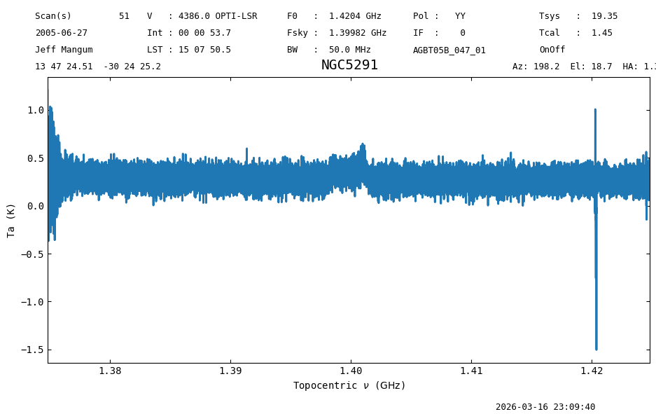
The default plot uses the frequency frame and Doppler convention found in the SDFITS file. In this case, that is topocentric frame (ITRS) and the optical convention. Notice that the GBT SDFITS file stores frequencies with CTYPE1=”FREQ-OBS”. Check by looking at sdfits[“CTYPE1”][0].

sdfits["CTYPE1"][0]

nan

ta.plot();

Although the spectrum ta can be printed using print, just printing it as an object gives some more information

print(ta)
print("\n")
ta

Spectrum (length=32768)
Flux=[0.2448421  0.31819268 0.19866335 ... 0.57650381 0.2179878
      1.20767879] K,  mean=0.28071 K
Spectral Axis=[1.42481684e+09 1.42481531e+09 1.42481379e+09 ...
               1.37482142e+09 1.37481989e+09 1.37481836e+09] Hz,  mean=1399817601.06055 Hz

<Spectrum(flux=[0.24484210085049396 ... 1.2076787931163384] K (shape=(32768,), mean=0.28071 K); spectral_axis=<SpectralAxis 
   (observer: <ITRS Coordinate (obstime=2005-06-27T02:05:58.000, location=(0.0, 0.0, 0.0) km): (x, y, z) in m
                  (882593.9465029, -4924896.36541728, 3943748.74743984)
               (v_x, v_y, v_z) in km / s
                  (0., 0., 0.)>
    target: <SkyCoord (FK5: equinox=J2000.000): (ra, dec, distance) in (deg, deg, kpc)
                (206.85210758, -30.40701531, 1000000.)
             (pm_ra_cosdec, pm_dec, radial_velocity) in (mas / yr, mas / yr, km / s)
                (0., 0., 4386.)>
    observer to target (computed from above):
      radial_velocity=4410.070039086893 km / s
      redshift=0.014820217767934851
    doppler_rest=1420405000.0 Hz
    doppler_convention=optical)
  [1.42481684e+09 1.42481531e+09 1.42481379e+09 ... 1.37482142e+09
 1.37481989e+09 1.37481836e+09] Hz> (length=32768))>

A large amount of information is also stores in the meta data, which is a python dictionary associated with the Spectrum. Here is how to access the meta data of a spectrum, where we use a python trick to make the dictionary shown in alphabetical order:

dict(sorted(ta.meta.items()))

{'AP_EFF': np.float64(0.6094633241501576),
 'AZIMUTH': 198.1588901992111,
 'BACKEND': 'Spectrometer',
 'BANDWID': 50000000.0,
 'BANDWIDTH': 50000000.0,
 'BINTABLE': 0,
 'BUNIT': 'K',
 'CAL': 'F',
 'CALPOSITION': 'Unknown',
 'CALTYPE': 'LOW',
 'CDELT1': -1525.87890625,
 'CRPIX1': 16385.0,
 'CRVAL1': 1399816838.1210938,
 'CRVAL2': np.float64(206.85210757719534),
 'CRVAL3': np.float64(-30.407015310885345),
 'CRVAL4': -6.0,
 'CTYPE1': 'FREQ-OBS',
 'CTYPE2': 'RA',
 'CTYPE3': 'DEC',
 'CTYPE4': 'STOKES',
 'CUNIT1': 'Hz',
 'CUNIT2': 'deg',
 'CUNIT3': 'deg',
 'DATE': '2005-06-27',
 'DATE-OBS': '2005-06-27T02:05:58.00',
 'DOPFREQ': 1420405000.0,
 'DURATION': np.float64(55.5225),
 'E2ESC': 0,
 'ELEVATIO': 18.69449298449073,
 'EQUINOX': 2000.0,
 'EXPOSURE': np.float64(53.7157844463702),
 'EXTEND': True,
 'EXTNAME': 'SINGLE DISH',
 'FDNUM': 0,
 'FEED': 1,
 'FEEDEOFF': 0.0,
 'FEEDXOFF': 0.0,
 'FILE': 'AGBT05B_047_01.raw.acs.fits',
 'FITSINDEX': 0,
 'FITSVER': '1.9',
 'FREQINT': -1525.878906,
 'FREQRES': 1846.3134765625,
 'FRONTEND': 'Rcvr1_2',
 'HDU': 1,
 'HUMIDITY': 0.754,
 'IFNUM': 0,
 'INDEX': 3,
 'INSTRUME': 'Spectrometer',
 'INTNUM': 0,
 'LASTOFF': 0.0,
 'LASTON': 51.0,
 'LST': 54470.49953792763,
 'MEANTSYS': np.float64(19.356765383560564),
 'NAXIS1': 32768,
 'NSAVE': -1,
 'NUMCHN': 32768,
 'OBJECT': 'NGC5291',
 'OBSERVER': 'Jeff Mangum',
 'OBSFREQ': 1399816838.1210938,
 'OBSID': 'unknown',
 'OBSMODE': 'OnOff:PSWITCHON:TPWCAL',
 'ORIGIN': 'NRAO Green Bank',
 'PLNUM': 0,
 'POL': 'YY',
 'PRESSURE': 697.7295162882529,
 'PROC': 'OnOff',
 'PROCSCAN': 'Unknown',
 'PROCSEQN': 1,
 'PROCSIZE': 2.0,
 'PROCTYPE': 'SIMPLE',
 'PROJID': 'AGBT05B_047_01',
 'QD_BAD': -1.0,
 'QD_EL': nan,
 'QD_METHOD': '',
 'QD_XEL': nan,
 'RADESYS': 'FK5',
 'RESTFREQ': 1420405000.0,
 'RESTFRQ': np.float64(1420405000.0),
 'ROW': 3,
 'RVSYS': 4376523.966595529,
 'SAMPLER': 'A13',
 'SCAN': 51,
 'SDFITVER': 'sdfits ver1.22',
 'SE_UNIT': 'micron',
 'SIDEBAND': 'U',
 'SIG': 'T',
 'SIMPLE': True,
 'SITEELEV': 824.595,
 'SITELAT': 38.43312,
 'SITELONG': -79.83983,
 'SRFEED': 0.0,
 'SUB': 1,
 'SUBREF_STATE': 1.0,
 'SURF_ERR': np.float64(440.0),
 'TAMBIENT': 292.54999999999995,
 'TCAL': np.float64(1.4526499509811401),
 'TCOLD': nan,
 'TDIM7': '(32768,1,1,1)',
 'TELESCOP': 'NRAO_GBT',
 'TIMESTAMP': '2005_06_27_02:05:58',
 'TRGTLAT': -30.407,
 'TRGTLONG': 206.85199999999995,
 'TSCALE': 'Ta',
 'TSCALFAC': np.float64(1.0),
 'TSYS': np.float64(19.353858908450768),
 'TUNIT7': 'K',
 'TWARM': nan,
 'VELDEF': 'OPTI-LSR',
 'VELOCITY': 4386000.0,
 'VFRAME': 22609.232181632025,
 'WCALPOS': 'Unknown',
 'WTTSYS': np.float64(19.353858908450764),
 'ZEROCHAN': 282.5385437011719}

For the remainder of the notebook, we focus on the small section of the spectrum near 1.39 GHz where a random spike can be seen in the previous plot. After some trial and error this is channel 21921 where the peak value is 0.59789101 K.

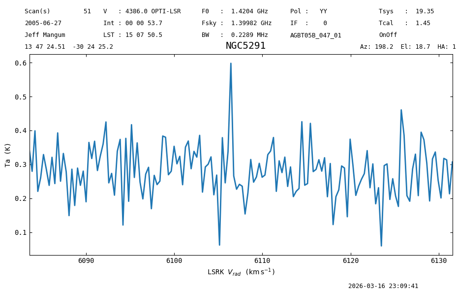
Let’s plot this zoomed spectrum in km/s so we can better see the effect of changing frames and conventions.

# pick a zoomed spectrum  (this cell is safe to re-execute)
if ta.nchan > 1000:
    print(f"Taking a zoomed spectrum")
    print(ta[21920:21923])   # print values around the spike, peak is at channel 21921
    ta = ta[21850:22000]     # these are the 150 channels we will zoom into
else:
    print(f"Already had the zoomed spectrum of {ta.nchan} channels")
    print(ta[70:73])         # peak is at channel 71

ta.plot(xaxis_unit='km/s')
print(f"Peak at {ta.velocity_axis_to('km/s')[71]} in the {ta.velocity_frame} reference frame")

Taking a zoomed spectrum
Spectrum (length=3)
Flux=[0.33822484 0.59789101 0.26609857] K,  mean=0.40074 K
Spectral Axis=[1.39136957e+09 1.39136805e+09 1.39136652e+09] Hz,  mean=1391368046.61719 Hz

Peak at 6256.475163870091 km / s in the itrs reference frame

Writing a spectrum

The default Spectrum.write uses its native units (Hz) to write a spectrum. Arguably more useful is the spectral axis in km/s. One way is to make a copy of the spectrum while changing the units, using Spectrum.with_spectral_axis_unit

But first a default write operation, with spectral axis in Hz:

# helper function to show the first few lines of a file
def head(filename, nlines=3):
    """ emulate the unix `head` program
    """
    with open(filename, 'r') as file:
        for i, line in enumerate(file, 1):
            print(line.strip())
            if i == nlines:
                break

spike_table = "output/ngc5291_spike.tab"

ta.write(spike_table,format="ascii.commented_header", overwrite=True)  
head(spike_table)

# spectral_axis flux uncertainty weight mask baseline
1391476384.0195374 0.34372934266958427 0.0 218.81991773344748 0 0.0
1391474858.1406312 0.27963123045821414 0.0 218.81991773344748 0 0.0

ta1 = ta.with_spectral_axis_unit("km/s")
ta1.write(spike_table,format="ascii.commented_header", overwrite=True)  
head(spike_table)

# spectral_axis flux uncertainty weight mask baseline
6232.646842534682 0.34372934266958427 0.0 218.75420976172921 0 0.0
6232.982426932439 0.27963123045821414 0.0 218.75420976172921 0 0.0

Change Rest Frame

You can change the velocity frame by supplying one of the built-in astropy coordinate frames. These are specified by a string name.

For example, to plot in the barycentric frame use "icrs". The change from topocentric to barycentric is small, about 25 km/s in this case.

ta.plot(vel_frame='icrs', xaxis_unit='km/s', grid=True);

Recall that the peak was at 6256.5 km/s in the topocentric frame, whereas in the barycentric frame it is more like 6231.9 km/s.

In addition to the astropy frame names, we also allow 'topo' and 'topocentric'.

ta.plot(vel_frame='topo', xaxis_unit='km/s');

Doppler Convention

One can also change the Doppler convention between radio, optical, and relativistic. Here we also change the x-axis to velocity units and use LSRK frame.

ta.plot(vel_frame='lsrk', doppler_convention='radio', xaxis_unit='km/s');

Changing the Spectral Axis of the Spectrum.

There are two ways to accomplish this. One returns a copy of the original Spectrum with the new spectral axis; the other changes the spectral axis in place.

The with_frame() and with_velocity_convention() are used when returning a copy. The two can be chained.

The set_frame() and set_convention() are used in place.

A. Return a copy of the spectrum using Spectrum.with_frame

newspec = ta.with_frame('galactocentric')
newspec.plot(xaxis_unit="km/s",doppler_convention='radio')

<dysh.plot.specplot.SpectrumPlot at 0x758f1c007df0>

print(f"The new spectral axis frame is {newspec.velocity_frame}")
print('radio:  ',newspec.velocity_axis_to("km/s", doppler_convention="radio")[71])     # 5976.1
print('default:',newspec.velocity_axis_to("km/s")[71],  newspec.velocity_convention)   # 6097.6

The new spectral axis frame is galactocentric
radio:   5976.071520424435 km / s
default: 6097.62168733356 km / s optical

One can see that the spectral axis of the new spectrum is different. About 722 kHz.

ta.spectral_axis - newspec.spectral_axis

\[[-722615.33,~-722614.54,~-722613.75,~\dots,~-722498.85,~-722498.05,~-722497.26] \; \mathrm{Hz}\]

B. Change the spectral axis in place using Spectrum.set_frame

print(ta.velocity_axis_to("km/s")[71]) # 6256.475
sa = ta.spectral_axis
ta.set_frame('gcrs')
print(f"Changed spectral axis frame to  {ta.velocity_frame}")
print(ta.velocity_axis_to("km/s")[71]) # 6256.365

6256.475163870091 km / s
Changed spectral axis frame to  gcrs
6256.365280719204 km / s

The difference between GCRS (geocentric) and ITRS (topocentric) is very small, a mere 0.110 km/s: 6256.475 vs. 6256.365 km/s

ta.plot(xaxis_unit="km/s");

Here the original the spectral axis has changed, albeit by a very small change.

500 Hz or 0.10 km/s

ta.spectral_axis - sa

\[[499.59287,~499.59232,~499.59177,~\dots,~499.51233,~499.51179,~499.51124] \; \mathrm{Hz}\]

ta.set_convention('radio')

ta.plot(xaxis_unit="km/s")
print(ta.velocity_axis_to("km/s")[71])

6128.470305969093 km / s

The target and observer are essential if you want to convert between different frames and conventions, as they control where on the sky and on earth the observations were taken resp.

ta.target

<SkyCoord (FK5: equinox=J2000.000): (ra, dec, distance) in (deg, deg, kpc)
    (206.85210758, -30.40701531, 1000000.)
 (pm_ra_cosdec, pm_dec, radial_velocity) in (mas / yr, mas / yr, km / s)
    (0., 0., 4386.)>

ta.observer

<GCRS Coordinate (obstime=2005-06-27T02:05:58.000, obsgeoloc=(0., 0., 0.) m, obsgeovel=(0., 0., 0.) m / s): (x, y, z) in m
    (-3418483.37116048, -3651331.51587568, 3945691.32972075)
 (v_x, v_y, v_z) in km / s
    (-4.3110922e-08, 9.51169059e-08, 6.55464828e-08)>

Other useful functions

Spectral Axis Conversion

Convert the spectral axis to any units, frame, and convention with Spectrum.velocity_axis_to.

dysh understands some common synonyms like ‘heliocentric’ for astropy’s ‘hcrs’. Note this returns an array, and does not modify the spectrum meta data.

ta.velocity_axis_to(unit="pc/Myr", toframe='heliocentric', doppler_convention='radio')

\[[6220.2727,~6220.6021,~6220.9315,~\dots,~6268.6937,~6269.0231,~6269.3525] \; \mathrm{\frac{pc}{Myr}}\]

Spectral Shift

Shift a spectrum in place to a given radial velocity or redshift with Spectrum.shift_spectrum_to

print(ta.velocity_axis_to("km/s")[71])

6128.470305969093 km / s

print(f"before shift {ta.spectral_axis[0]}...")
ta.shift_spectrum_to(radial_velocity=0*u.km/u.s)
print(f"after shift {ta.spectral_axis[0]}...")

before shift 1391476883.6124058 Hz...
after shift 1412098366.9399488 Hz...

Spectral Axis in Wavelengths

The default is angstrom, use Quantity.to to convert to other units.

ta.wavelength.to('cm')

\[[21.230281,~21.230305,~21.230328,~\dots,~21.233704,~21.233728,~21.233751] \; \mathrm{cm}\]

Plot in Channels

Also, you can plot the x-axis in channel units

ta.plot(xaxis_unit='chan');

Final Stats

Finally, at the end we compute some statistics over a spectrum, merely as a checksum if the notebook is reproducible.

ta.check_stats(0.07586939 * u.K)

23:09:42.734 I rms is OK