# These modules are required for this example.
import numpy as np
import astropy.units as u
from dysh.spectra import tsys_weight
from dysh.spectra import average_spectra
from dysh.fits.gbtfitsload import GBTFITSLoad
from dysh.log import init_logging

# These modules are used for file I/O
from dysh.util.files import dysh_data
from pathlib import Path

Using Spectral Weights

This notebook shows how to weigh Scans and Spectra during averaging and how to find out what weights were used in the process.

Dysh commands

The following dysh commands are introduced (leaving out all the function arguments):

filename = dysh_data()
sdf = GBTFITSLoad()
sdf.select()
sb = sdf.getps()
ta = sb.timeaverage()
ta.baseline()
ta.average()
ta.plot()
tsys_weight

Loading Modules

We start by loading the modules we will use for the data reduction.

Setup

We start the dysh logging, so we get more information about what is happening. This is only needed if working on a notebook. If using the CLI through the dysh command, then logging is setup for you.

init_logging(2)

# also create a local "output" directory where temporary notebook files can be stored.
output_dir = Path.cwd() / "output"
output_dir.mkdir(exist_ok=True)

Data Retrieval

Download the example SDFITS data, if necessary.

filename = dysh_data(test="getps")

23:09:15.022 I Resolving test=getps -> AGBT05B_047_01/AGBT05B_047_01.raw.acs/

Data Loading

Next, we use GBTFITSLoad to load the data, and then its summary method to inspect its contents.

sdf = GBTFITSLoad(filename)
sdf.summary()

23:09:15.073 I Index loaded from .index file (44/93 columns). Missing columns (TCAL, WCS, calibration metadata, etc.) will be automatically loaded from FITS file when first accessed.

SCAN	OBJECT	VELOCITY	PROC	PROCSEQN	RESTFREQ	# IF	# POL	# INT	# FEED	AZIMUTH	ELEVATION
51	NGC5291	4386.0	OnOff	1	1.420405	1	2	11	1	198.3431	18.6427
52	NGC5291	4386.0	OnOff	2	1.420405	1	2	11	1	198.9306	18.7872
53	NGC5291	4386.0	OnOff	1	1.420405	1	2	11	1	199.3305	18.3561
54	NGC5291	4386.0	OnOff	2	1.420405	1	2	11	1	199.9157	18.4927
55	NGC5291	4386.0	OnOff	1	1.420405	1	2	11	1	200.3042	18.0575
56	NGC5291	4386.0	OnOff	2	1.420405	1	2	11	1	200.8906	18.1860
57	NGC5291	4386.0	OnOff	1	1.420405	1	2	11	1	202.3275	17.3853
58	NGC5291	4386.0	OnOff	2	1.420405	1	2	11	1	202.9192	17.4949

Position Switched Calibration

We calibrate several scans at once for NGC5291. This results in a ScanBlock with 4 scans, each with 11 integrations. The default weights are unity, with one weight value per integration.

pssb = sdf.getps(object='NGC5291', ifnum=0, plnum=1, fdnum=0)
print(f"Number of scans: {len(pssb)}, Number of integrations per scan: {[k.nint for k in pssb]}")
print(f"Scan weights: {pssb.weights}")

Number of scans: 4, Number of integrations per scan: [11, 11, 11, 11]
Scan weights: [array([1., 1., 1., 1., 1., 1., 1., 1., 1., 1., 1.]), array([1., 1., 1., 1., 1., 1., 1., 1., 1., 1., 1.]), array([1., 1., 1., 1., 1., 1., 1., 1., 1., 1., 1.]), array([1., 1., 1., 1., 1., 1., 1., 1., 1., 1., 1.])]

Applying weights when averaging Scans

When time averaging integrations and/or scans to create a final spectrum, you can choose from dysh’s two options (‘tsys’ or None) or supply your own weight array.

1. System temperature weighting

The default for timeaverage is ‘tsys’ which calculates and applies system temperature weighting to each integration:

\[ w = t_{exp} \times \delta\nu/T_{sys}^2 \]

where \(t_{exp}\) is the integration exposure time, \(\delta\nu\) is the channel width, and \(T_{sys}\) is the system temperature. You can check what those weights will be with tsys_weight.

pssb.tsys_weight

array([array([20.02238592, 19.23775753, 19.89469281, 19.13748516, 19.43619207,
              19.24989036, 19.94781504, 19.81766121, 19.90398672, 19.86791497,
              19.1754635 ])                                                   ,
       array([18.94476267, 19.78439063, 19.85434244, 19.90054628, 19.95968097,
              19.08878802, 18.97575899, 18.5760123 , 19.76114768, 19.71441725,
              19.70968407])                                                   ,
       array([18.77161334, 19.62257845, 19.70200273, 19.68613794, 19.65882906,
              19.85660591, 19.57284449, 19.60902436, 18.74157248, 18.6538321 ,
              18.75593527])                                                   ,
       array([18.44256036, 18.36839774, 18.34613799, 18.39603826, 17.95338427,
              19.04965151, 19.09771163, 19.18475276, 19.09809603, 19.09126971,
              18.34217249])                                                   ],
      dtype=object)

Technical note: this is an array of arrays rather than a multidimensional array because different scans may have differing numbers of integrations.

timeaverage with the default arguments will use these weights. The final spectral weight is the sum of all weights.

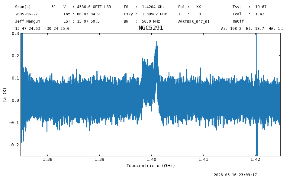
In the following lines of code we will time average the \(4\times11\) integrations using the default weights (‘tsys’), and then remove a baseline from the resulting time average. For the baseline removal we exclude ranges at the edges of the spectrum and where we know there’s a signal. We end by plotting the time averged baseline subtracted spectrum, and printing the weights and statistics.

ta1 = pssb.timeaverage()  # default is weights='tsys'

# Define regions to be excluded from the baseline fit.
exclude_regions = [(1.37*u.GHz,1.38*u.GHz),
                   (1.395*u.GHz,1.405*u.GHz),
                   (1.42*u.GHz,1.43*u.GHz)]

# Fit an order 1 polynomial excluding the ranges defined above and subtract it (remove=True).
ta1.baseline(degree=1, remove=True, exclude=exclude_regions)

# Plot the result.
ta1.plot(ymin=-0.25, ymax=0.3)

# Print final weights and statistics.
print(f"final weights={ta1.weights}")
ta1.stats()  # rms 0.05926608 K

23:09:16.517 I 1370000000.0 Hz is below the minimum spectral axis 1374818364.0 Hz. Replacing.

23:09:16.517 I 1430000000.0 Hz is above the maximum spectral axis 1424816838.1210938 Hz. Replacing.

23:09:16.519 I EXCLUDING [Spectral Region, 1 sub-regions:
  (1374818364.0 Hz, 1380000000.0 Hz) 
, Spectral Region, 1 sub-regions:
  (1395000000.0 Hz, 1405000000.0 Hz) 
, Spectral Region, 1 sub-regions:
  (1420000000.0 Hz, 1424816838.1210938 Hz) 
]

final weights=[847.9619254640448 847.9619254640448 847.9619254640448 ...
 847.9619254640448 847.9619254640448 847.9619254640448]

{'mean': <Quantity 0.00493475 K>,
 'median': <Quantity 0.00348282 K>,
 'rms': <Quantity 0.05926608 K>,
 'min': <Quantity -1.74795385 K>,
 'max': <Quantity 0.76657302 K>,
 'npt': 32768,
 'nan': np.int64(0)}

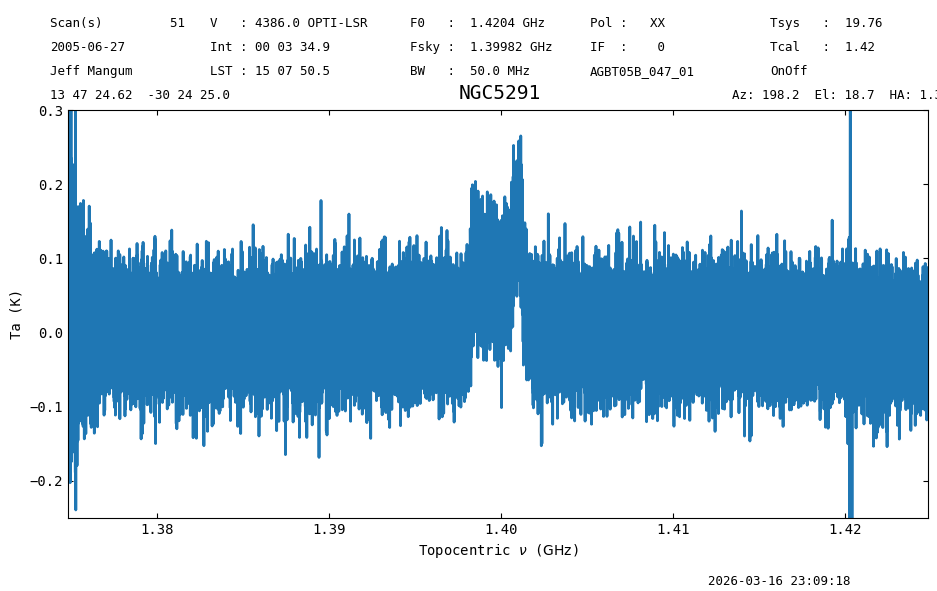
2. Equal weighting

Supplying weights=None will weight all integrations the same. In this case, the result is not much different than tsys, because the \(T_{sys}\) weights were already pretty uniform. We also baseline subtract and plot the results.

ta2 = pssb.timeaverage(weights=None)  
ta2.baseline(degree=1, remove=True, exclude=exclude_regions)
ta2.plot(ymin=-0.25, ymax=0.3)
print(f"final weights={ta2.weights}")
ta2.stats() # rms 0.05928395 K

23:09:17.394 I 1370000000.0 Hz is below the minimum spectral axis 1374818364.0 Hz. Replacing.

23:09:17.395 I 1430000000.0 Hz is above the maximum spectral axis 1424816838.1210938 Hz. Replacing.

23:09:17.397 I EXCLUDING [Spectral Region, 1 sub-regions:
  (1374818364.0 Hz, 1380000000.0 Hz) 
, Spectral Region, 1 sub-regions:
  (1395000000.0 Hz, 1405000000.0 Hz) 
, Spectral Region, 1 sub-regions:
  (1420000000.0 Hz, 1424816838.1210938 Hz) 
]

final weights=[4.0 4.0 4.0 ... 4.0 4.0 4.0]

{'mean': <Quantity 0.00493513 K>,
 'median': <Quantity 0.00344473 K>,
 'rms': <Quantity 0.05928395 K>,
 'min': <Quantity -1.74943676 K>,
 'max': <Quantity 0.76626611 K>,
 'npt': 32768,
 'nan': np.int64(0)}

3. User-supplied weights

You can supply a numpy array of weights to apply. For ScanBlock.timeaverage the weights must have shape (Nint,) or (Nint,nchan) where Nint is the number of integrations in the ScanBlock and nchan is the number of channels in each scan.

3a. Number of weights equal to number of integrations

We create a slightly silly example, that weights later integrations more.

w = np.arange(1, pssb.nint+1, dtype=float)
ta3a = pssb.timeaverage(weights=w)
ta3a.baseline(degree=1, remove=True, exclude=exclude_regions)
ta3a.plot(ymin=-0.25, ymax=0.3)
print(f"final weights={ta3a.weights}")

23:09:18.079 I 1370000000.0 Hz is below the minimum spectral axis 1374818364.0 Hz. Replacing.

23:09:18.080 I 1430000000.0 Hz is above the maximum spectral axis 1424816838.1210938 Hz. Replacing.

23:09:18.081 I EXCLUDING [Spectral Region, 1 sub-regions:
  (1374818364.0 Hz, 1380000000.0 Hz) 
, Spectral Region, 1 sub-regions:
  (1395000000.0 Hz, 1405000000.0 Hz) 
, Spectral Region, 1 sub-regions:
  (1420000000.0 Hz, 1424816838.1210938 Hz) 
]

final weights=[990.0 990.0 990.0 ... 990.0 990.0 990.0]

3b. Weights for each channel and integration

Supposed you had a channel-based \(T_{sys}\) for each integration and wanted to calculate and apply system temperature weights. This can be accomplished by giving a weights array to ScanBlock.timeaverage.

First we fake a tsys array of the correct shape. Then we calculate system temperate weights using the mean exposure time and mean channel width of the scans.

np.random.seed(123)  # make sure we have a fixed seed
tsys = 30 + np.random.rand(pssb.nint, pssb.nchan)*15.0  # Fake system temperature array in the 30-45K range.
# The mean exposure and channel width.
dt = np.mean(np.mean(pssb.exposure))
df = np.mean(np.mean(pssb.delta_freq))

# Compute new weights using the inverse variance as given by the radiometer equation.
w = tsys_weight(dt, df, tsys)
print(f"{tsys=}")
print(f"Weights array shape: {w.shape}")

tsys=array([[40.44703778, 34.29209002, 33.4027718 , ..., 38.71791603,
        35.28713315, 40.87063212],
       [38.05088391, 33.34662369, 42.20490842, ..., 41.80063624,
        38.89300609, 40.57733459],
       [35.43088049, 39.82836535, 33.14689888, ..., 33.44782766,
        40.81104733, 34.50116723],
       ...,
       [44.27286605, 40.55077356, 32.97672831, ..., 40.44991244,
        31.97284355, 39.87806732],
       [43.54054032, 37.95174176, 36.0192332 , ..., 30.24616871,
        32.32690178, 40.55712875],
       [31.4013107 , 36.35880619, 38.0259688 , ..., 34.22566874,
        42.53679606, 40.73033967]], shape=(44, 32768))
Weights array shape: (44, 32768)

Now time average the data using the weights defined above, and repeat the baseline subtraction and plotting.

ta3b = pssb.timeaverage(weights=w)
ta3b.baseline(degree=1, remove=True, exclude=exclude_regions)
ta3b.plot(ymin=-0.25, ymax=0.3)
print(f"final weights={ta3b.weights}")

23:09:18.926 I 1370000000.0 Hz is below the minimum spectral axis 1374818364.0 Hz. Replacing.

23:09:18.927 I 1430000000.0 Hz is above the maximum spectral axis 1424816838.1210938 Hz. Replacing.

23:09:18.928 I EXCLUDING [Spectral Region, 1 sub-regions:
  (1374818364.0 Hz, 1380000000.0 Hz) 
, Spectral Region, 1 sub-regions:
  (1395000000.0 Hz, 1405000000.0 Hz) 
, Spectral Region, 1 sub-regions:
  (1420000000.0 Hz, 1424816838.1210938 Hz) 
]

final weights=[243.4369815211293 245.3675937036399 237.113209395157 ...
 242.4000731446227 249.68128171631173 237.80401320732614]

Note the scan weights have been updated, and are now equal to the weights supplied to the timeaverage function, so their shape is now (nint, nchan).

print(pssb[0].weights.shape)
print(f"Are the Scan weights the same as those we defined? {np.all(w[0:11] == pssb[0].weights)}")

(11, 32768)
Are the Scan weights the same as those we defined? True

Applying weights when averaging Spectrum

The method average_spectra can compute weighted averages in 3 ways. The first two are the usual weights='tsys' and weights=None options. The third option, weights='spectral' will average the spectra using the values in each of their weights array. Note that average_spectra is the function used by Spectrum.average to average spectra.

sp = average_spectra([ta1, ta2, ta3a, ta3b], weights='spectral')

# but this is the same:
# sp = ta1.average([ ta2, ta3a, ta3b], weights='spectral')

sp.plot(ymin=-0.25, ymax=0.3)
print(f"final weights={sp.weights}")

final weights=[2085.398906985174 2087.329519167685 2079.0751348592016 ...
 2084.3619986086674 2091.6432071803565 2079.765938671371]

Final Stats

Finally, at the end we compute some statistics over a spectrum, merely as a checksum if the notebook is reproducible.

sp.check_stats(0.06025871 * u.K)

23:09:19.729 I rms is OK