Saving Data to External Files#
This notebook gives examples of how to write out selected data from GBTFitsLoad and how to save Spectrum, Scan, and ScanBlock to different formats. It also introduces the dysh_data function to obtain filename references to various test and example data.
Dysh Commands#
The following dysh commands are introduced (leaving out all the function arguments):
filename = dysh_data()
sdf = GBTFITSLoad()
sb = sdf.getps()
ta = sb.timeaverage()
ta.average()
ta.plot()
ta.write()
Spectrum.read()
Loading Modules#
We start by loading the modules we will use for this example.
For display purposes, we use the static (non-interactive) matplotlib backend in this tutorial. However, you can tell matplotlib to use the ipympl backend to enable interactive plots. This is only needed if working on jupyter lab or notebook.
# These modules are required for loading and reading data.
from dysh.fits.gbtfitsload import GBTFITSLoad
from dysh.spectra.spectrum import Spectrum
from astropy import units as u
from dysh.log import init_logging

# We will use matplotlib for plotting.
import matplotlib.pyplot as plt

# These modules are used for file I/O
from dysh.util.files import dysh_data
from pathlib import Path
Setup#
We start the dysh logging, so we get more information about what is happening.
This is only needed if working on a notebook.
If using the CLI through the dysh command, then logging is setup for you.
We also create a directory where output files from the notebook get stored.
init_logging(2)

# also create a local "output" directory where temporary notebook files can be stored.
output_dir = Path.cwd() / "output"
output_dir.mkdir(exist_ok=True)
Data Retrieval#
Download the example SDFITS data, if necessary.
The actual full path filename will depend on your dysh installation, it could be local, or it will need to be downloaded.
The
dysh_data
function has a few mnemonics, to avoid having to remember long filenames. Data via test= are available for developers, since they come with the code. Data via example= will need to be downloaded, unless you have downloaded the example data into $DYSH_DATA/example_data.
Here is an example how to find the aliases available with test=
dysh_data(test="?")
# dysh_data::test
# ---------------
getps AGBT05B_047_01/AGBT05B_047_01.raw.acs/
getps2 TGBT21A_501_11/TGBT21A_501_11.raw.vegas.fits
getfs TGBT21A_504_01/TGBT21A_504_01.raw.vegas/TGBT21A_504_01.raw.vegas.A.fits
subbeamnod2 TRCO_230413_Ka
For many example notebooks we use the test="getps" dataset. In the next cell there are multiple ways to get at the same data:
# filename = dysh_data(example="positionswitch/data/AGBT05B_047_01/AGBT05B_047_01.raw.acs/AGBT05B_047_01.raw.acs.fits")
# filename = dysh_data(example="getps")
filename = dysh_data(test="getps")
23:05:02.487 I Resolving test=getps -> AGBT05B_047_01/AGBT05B_047_01.raw.acs/
Data Loading#
Next, we use GBTFITSLoad to load the data, and report some basic info and use the summary method to inspect its contents.
sdfits = GBTFITSLoad(filename)
sdfits.info()
23:05:02.541 I Index loaded from .index file (44/93 columns). Missing columns (TCAL, WCS, calibration metadata, etc.) will be automatically loaded from FITS file when first accessed.
Filename: /home/docs/checkouts/readthedocs.org/user_builds/dysh/checkouts/release-1.0.0/testdata/AGBT05B_047_01/AGBT05B_047_01.raw.acs/AGBT05B_047_01.raw.acs.fits
No.    Name      Ver    Type      Cards   Dimensions   Format
  0  PRIMARY       1 PrimaryHDU      12   ()
  1  SINGLE DISH    1 BinTableHDU    229   352R x 70C   [32A, 1D, 22A, 1D, 1D, 1D, 32768E, 16A, 6A, 8A, 1D, 1D, 1D, 4A, 1D, 4A, 1D, 1I, 32A, 32A, 1J, 32A, 16A, 1E, 8A, 1D, 1D, 1D, 1D, 1D, 1D, 1D, 1D, 1D, 1D, 1D, 1D, 8A, 1D, 1D, 12A, 1I, 1I, 1D, 1D, 1I, 1A, 1I, 1I, 16A, 16A, 1J, 1J, 22A, 1D, 1D, 1I, 1A, 1D, 1E, 1D, 1A, 1A, 8A, 1E, 1E, 16A, 1I, 1I, 1I]
sdfits.summary()
| SCAN | OBJECT | VELOCITY | PROC | PROCSEQN | RESTFREQ | # IF | # POL | # INT | # FEED | AZIMUTH | ELEVATION |
|---|---|---|---|---|---|---|---|---|---|---|---|
| 51 | NGC5291 | 4386.0 | OnOff | 1 | 1.420405 | 1 | 2 | 11 | 1 | 198.3431 | 18.6427 |
| 52 | NGC5291 | 4386.0 | OnOff | 2 | 1.420405 | 1 | 2 | 11 | 1 | 198.9306 | 18.7872 |
| 53 | NGC5291 | 4386.0 | OnOff | 1 | 1.420405 | 1 | 2 | 11 | 1 | 199.3305 | 18.3561 |
| 54 | NGC5291 | 4386.0 | OnOff | 2 | 1.420405 | 1 | 2 | 11 | 1 | 199.9157 | 18.4927 |
| 55 | NGC5291 | 4386.0 | OnOff | 1 | 1.420405 | 1 | 2 | 11 | 1 | 200.3042 | 18.0575 |
| 56 | NGC5291 | 4386.0 | OnOff | 2 | 1.420405 | 1 | 2 | 11 | 1 | 200.8906 | 18.1860 |
| 57 | NGC5291 | 4386.0 | OnOff | 1 | 1.420405 | 1 | 2 | 11 | 1 | 202.3275 | 17.3853 |
| 58 | NGC5291 | 4386.0 | OnOff | 2 | 1.420405 | 1 | 2 | 11 | 1 | 202.9192 | 17.4949 |
Calibrate a position switched scan#
The getps function returns a ScanBlock containing one PSScan with 11 integrations for the ON position and 11 integrations for the OFF position.
ps_scan_block = sdfits.getps(scan=51, ifnum=0, plnum=0, fdnum=0)
print(f"Number of integrations = {ps_scan_block[0].nrows}")
Number of integrations = 22
Get the time average of the calibrated data. This method returns a Spectrum.
ta = ps_scan_block.timeaverage()
ta.plot();
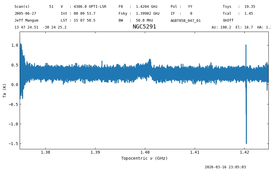
In the Position-Switched Data Reduction notebook we will go in more depth on this particular data. Here we continue with some examples of how to write and read data.
Reading and Writing Individual Spectra#
Inputs and Outputs#
dysh supports output to text files in a variety of formats familiar to users of astropy:
basic
commented_header
ECSV
fixed_width
IPAC
MRT
votable
The following lines of code define some of the available formats in a list, and then loop over them saving the calibrated data in each format.
We use the overwrite=True parameter to avoid errors if the files already exist on disk.
# Define the formats in a list.
fmt = [
    "basic",
    "commented_header",
    "ecsv",
    "fixed_width",
    "ipac",
    "mrt",
    "votable",
]


# Loop over formats writing the calibrated spectrum.
for f in fmt:
    file = output_dir / f"testwrite.{f}"
    ta.write(file, format=f, overwrite=True)
We can also write a Spectrum to FITS format
NOTE: this is actually NOT the SDFITS format, but a BINTABLE erroneously labeled as “SINGLE DISH”.
ta.write(output_dir / "testwrite.fits", format="fits", overwrite=True)
WARNING: Attribute `QD_XEL` of type <class 'float'> cannot be added to FITS Header - skipping [astropy.io.fits.convenience]
WARNING: Attribute `QD_EL` of type <class 'float'> cannot be added to FITS Header - skipping [astropy.io.fits.convenience]
WARNING: Attribute `TWARM` of type <class 'float'> cannot be added to FITS Header - skipping [astropy.io.fits.convenience]
WARNING: Attribute `TCOLD` of type <class 'float'> cannot be added to FITS Header - skipping [astropy.io.fits.convenience]
We can read spectra in FITS and a few formats. As noted in astropy, ECSV is the only ASCII format that can make a lossless output-input roundtrip and thus reproduce an original spectrum.
We use the Spectrum.read method to read the saved data.
s1 = Spectrum.read(output_dir / "testwrite.fits", format="fits")
s1.plot();

s2 = Spectrum.read(output_dir / "testwrite.ecsv", format="ecsv")
s2.plot();
GBTIDL ASCII format#
dysh can read text files created by GBTIDL’s write_ascii function. However, those files do not provide sufficient metadata to fully recreate the spectrum.
# "https://www.gb.nrao.edu/dysh/example_data/onoff-L/gbtidl-data/onoff-L_gettp_156_intnum_0_HEL.ascii"
filename_ascii = dysh_data(example="onoff-L/gbtidl-data/onoff-L_gettp_156_intnum_0_HEL.ascii")
s3 = Spectrum.read(filename_ascii, format='gbtidl')
23:05:09.944 I url: http://www.gb.nrao.edu/dysh//example_data/onoff-L/gbtidl-data/onoff-L_gettp_156_intnum_0_HEL.ascii
Downloading onoff-L_gettp_156_intnum_0_HEL.ascii from http://www.gb.nrao.edu/dysh//example_data/onoff-L/gbtidl-data/onoff-L_gettp_156_intnum_0_HEL.ascii
23:05:10.361 I Starting download...
23:05:10.647 I Saved onoff-L_gettp_156_intnum_0_HEL.ascii to onoff-L_gettp_156_intnum_0_HEL.ascii
Retrieved onoff-L_gettp_156_intnum_0_HEL.ascii
print(s3, "\n", s3.meta)
Spectrum (length=32768)
Flux=[3608710. 3553598. 3604808. ... 3523171. 3545982. 3474847.] ct,  mean=493422767.43425 ct
Spectral Axis=[1.42009237 1.42009166 1.42009094 ... 1.39665654 1.39665582
               1.39665511] GHz,  mean=1.40837 GHz
 {'SCAN': 156, 'OBJECT': 'NGC2782', 'DATE-OBS': '2021-02-10 00:00:00.000', 'RA': np.float64(119.42083333333332), 'VELDEF': 'None-HEL', 'POL': 'YY'}
dysh can even read compressed ASCII files. Note these data have velocity on the spectral axis.
filename_ascii_gz = dysh_data(example="onoff-L/gbtidl-data/onoff-L_getps_152_RADI-HEL.ascii.gz")
s4 = Spectrum.read(filename_ascii_gz, format='gbtidl')
23:05:10.724 I url: http://www.gb.nrao.edu/dysh//example_data/onoff-L/gbtidl-data/onoff-L_getps_152_RADI-HEL.ascii.gz
Downloading onoff-L_getps_152_RADI-HEL.ascii.gz from http://www.gb.nrao.edu/dysh//example_data/onoff-L/gbtidl-data/onoff-L_getps_152_RADI-HEL.ascii.gz
23:05:10.966 I Starting download...
23:05:11.140 I Saved onoff-L_getps_152_RADI-HEL.ascii.gz to onoff-L_getps_152_RADI-HEL.ascii.gz
Retrieved onoff-L_getps_152_RADI-HEL.ascii.gz
print(s4, "\n", s4.meta)
Spectrum (length=32768)
Flux=[-0.1042543   0.05250004  0.00432693 ... -0.05038555  0.03408394
       0.06139921] K,  mean=0.17345 K
Spectral Axis=[1281.15245599 1281.30342637 1281.45439674 ... 6227.69690405
               6227.84787443 6227.99884481] km / s,  mean=3754.57565 km / s
 {'SCAN': 152, 'OBJECT': 'NGC2415', 'DATE-OBS': '2021-02-10 00:00:00.000', 'RA': np.float64(114.65624999999999), 'VELDEF': 'RADI-HEL', 'POL': 'YY'}
Plot#
To plot the spectrum contained in the ascii files you have to use matplotlib.
# set the rest frequency to the HI line
s4.rest_value = 1420405751.786 * u.Hz
plt.figure()
plt.xlabel(f"Velocity ({s4.meta['VELDEF']}) [{s4.spectral_axis.unit}]")
plt.ylabel(f"$T_A$ [{s4.flux.unit}]")
plt.plot(s4.spectral_axis, s4.flux);
/home/docs/checkouts/readthedocs.org/user_builds/dysh/envs/release-1.0.0/lib/python3.10/site-packages/traitlets/traitlets.py:1385: DeprecationWarning: Passing unrecognized arguments to super(Toolbar).__init__().
NavigationToolbar2WebAgg.__init__() missing 1 required positional argument: 'canvas'
This is deprecated in traitlets 4.2.This error will be raised in a future release of traitlets.
  warn(
Apart from the signal around 3800 km/s, there are a handfull of positive-negative instrumental spikes That is for another notebook.
Writing Multiple Calibrated Spectra to SDFITS#
You can write the calibrated data from a ScanBlock to the SDFITS format.
If there are multiple scans in the ScanBlock, they will all be written to the same SDFITS (useful for gbtgridder).
ps_scan_block.write(output_dir / "scanblock.fits", overwrite=True)
Reading Calibrated SDFITS#
To load the saved data, we use the same function we used to load the raw data, GBTFITSLoad.
ps_scan_block_read = GBTFITSLoad(output_dir / "scanblock.fits")
This is treated the same was as the raw data, so the same methods are available.
ps_scan_block_read.summary()
| SCAN | OBJECT | VELOCITY | PROC | PROCSEQN | RESTFREQ | # IF | # POL | # INT | # FEED | AZIMUTH | ELEVATION |
|---|---|---|---|---|---|---|---|---|---|---|---|
| 51 | NGC5291 | 4386.0 | OnOff | 1 | 1.420405 | 1 | 1 | 11 | 1 | 198.3431 | 18.6427 |
However, since the data is already calibrated, trying to fetch the data using calibration methods like getps or getnod will result in errors.
Instead, we can use the gettp method or getspec.
Using gettp#
If we use gettp, then we will get all of the integrations as a ScanBlock object.
tp_read = ps_scan_block_read.gettp(scan=51, ifnum=0, plnum=0, fdnum=0)
print(f"Number of integrations: {tp_read[0].nint}")
23:05:11.558 I Using TSYS column
Number of integrations: 11
We can access individual integration through the getspec method.
ta_read_0a = tp_read[0].getspec(0)
ta_read_0a.plot();
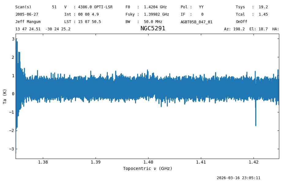
Using getspec#
Now we do the same using getspec. This method takes as input the row number we want to retrieve.
ta_read_0b = ps_scan_block_read.getspec(0)
ta_read_0b.plot();

If we take the difference, it is zero.
(ta_read_0a.data - ta_read_0b.data).sum()
np.float64(0.0)
Writing Out Selected Data from GBTFITSLoad#
The write method of GBTFITSLoad supports down-selection of data.
Data can be selected on any SDFITS column.
In the following call to GBTFITSLoad.write we will select a single polarization (plnum=1), and only the first five integrations of each scan (intnum=range(5)). We also set overwrite=True to avoid errors if the file already exists, and request that the output be saved into a single file (multifile=False).
sdfits.write(output_dir / "mydata.fits", plnum=1,
             intnum=range(5), overwrite=True, multifile=False)
23:05:12.426 I write: bintable 0: 80 rows, 32768 channels, 1 chunk(s) of 5000
23:05:12.457 I write: chunk [0:80] of 80 rows built (0.0s)
23:05:12.474 I write: chunk written to disk (0.0s)
 ID    TAG    PLNUM   INTNUM   # SELECTED
--- --------- ----- ---------- ----------
  0 4b46a8429     1 range(0,5)         80
These data, can of course, be read back in.
sdfits2 = GBTFITSLoad(output_dir / "mydata.fits")
sdfits2.summary()
| SCAN | OBJECT | VELOCITY | PROC | PROCSEQN | RESTFREQ | # IF | # POL | # INT | # FEED | AZIMUTH | ELEVATION |
|---|---|---|---|---|---|---|---|---|---|---|---|
| 51 | NGC5291 | 4386.0 | OnOff | 1 | 1.420405 | 1 | 1 | 5 | 1 | 198.2327 | 18.6739 |
| 52 | NGC5291 | 4386.0 | OnOff | 2 | 1.420405 | 1 | 1 | 5 | 1 | 198.8200 | 18.8193 |
| 53 | NGC5291 | 4386.0 | OnOff | 1 | 1.420405 | 1 | 1 | 5 | 1 | 199.2207 | 18.3889 |
| 54 | NGC5291 | 4386.0 | OnOff | 2 | 1.420405 | 1 | 1 | 5 | 1 | 199.8058 | 18.5264 |
| 55 | NGC5291 | 4386.0 | OnOff | 1 | 1.420405 | 1 | 1 | 5 | 1 | 200.1952 | 18.0919 |
| 56 | NGC5291 | 4386.0 | OnOff | 2 | 1.420405 | 1 | 1 | 5 | 1 | 200.7815 | 18.2213 |
| 57 | NGC5291 | 4386.0 | OnOff | 1 | 1.420405 | 1 | 1 | 5 | 1 | 202.2201 | 17.4228 |
| 58 | NGC5291 | 4386.0 | OnOff | 2 | 1.420405 | 1 | 1 | 5 | 1 | 202.8117 | 17.5334 |
Writing SDFITS to Multiple Files#
If the data came from multiple files, for instance VEGAS banks, then by default they are written to multiple files, so
sdfits.write('mydata.fits')
would write to mydata0.fits, mydata1.fits, … mydataN.fits.
If you want them organized for GBTFITSLoad, create a new directory first (and/or make sure this directory is clean):
   import os
   os.mkdir("my")
   sdfits.write("my/data.fits")
which would write my/data0.fits, my/data1.fits, … my/dataN.fits. This way GBTFITSLoad can more easily read them as a related group:
mysdf = GBTFITSLoad("my")
See also the Merging SDFITS Files notebook how to deal merging SDFITS files.
Final Stats#
Finally, at the end we compute some statistics over a spectrum, merely as a checksum if the notebook is reproducible.
ta_read_0a.check_stats(0.26165166 * u.K)
23:05:12.566 I rms is OK