Spectral Line Search

Spectral Line Search#

This notebook shows how to use dysh to search for spectral lines. Searches can be done for a user-specified frequency range or for the frequency axis of a Spectrum. You can use a remote query to Splatalogue or use local tables distributed with dysh.

First we show how to do a search using a SpectralLineSearch object, then using a Spectrum object. Examples are given both with and without a redshift value.

Dysh commands#

The following dysh commands are introduced (leaving out all the function arguments):

  tbl1 = SpectralLineSearch.query_lines()
  tbl2 = SpectralLineSearch.recomb()
  tbl3 = SpectralLineSearch.recomball()
  SpectralLineSearch.clear_cache()

  sp = Spectrum.fake_spectrum()
  sp.plot()
  sp.recomb()
  sp.query_lines()

Loading Modules#

We start by loading the modules we will use.

# These modules are required for this example.
from dysh.line import SpectralLineSearch
from dysh.spectra import Spectrum
from dysh.log import init_logging
from astropy import units as u
# These modules are used for file I/O
from dysh.util.files import dysh_data
from pathlib import Path

Setup#

dysh uses a logger to communicate. If you are working in the command line, then the logging is setup for you. If you are working in a jupyter lab instance, then you need to set it up. You can do so using the init_logging function imported above. As an argument, init_logging takes a number, the verbosity level. level 0 is for error messages only, 1 for warning, 2 for info and 3 for debug. Here we set it to level 2.

init_logging(2)

# also create a local "output" directory where temporary notebook files can be stored.
output_dir = Path.cwd() / "output"
output_dir.mkdir(exist_ok=True)

Example 1. Doing an online or local search with SpectralLineSearch#

SpectralLineSearch is a thin wrapper on top of astroquery.splatalogue.Splatalogue, with some additional conveniences for working in dysh and with GBT data. You search a catalog in a given frequency range, optionally narrow down to specific molecules, line strengths, energies, etc. The return object is an astropy Table. Below are a few example searches.

Do an online search for N2H+ lines between 80 and 400 GHz#

Online searching of Splatalogue is the default. Note in this example we use an initial space in the chemical_name to eliminate other molecules that have the string 'N2H+' in them. We set an intensity_lower_limit to weed out some of the weaker satellite lines. When giving an intensity_lower_limit, one must also provide an intensity_type string, a minimum match to 'CDMS/JPL (log)', 'Sij-mu2', or 'Aij (log)'.

minfreq = 80*u.GHz
maxfreq = 400*u.GHz
table = SpectralLineSearch.query_lines(minfreq, maxfreq, 
                                       chemical_name=" N2H+", 
                                       intensity_lower_limit=-3, 
                                       intensity_type="CDMS")

print(f"{len(table)} rows returned.")

57 rows returned.

To inspect the available columns use the Table.colnames attribute:

print(table.colnames)

['species_id', 'name', 'chemical_name', 'resolved_QNs', 'linelist', 'LovasASTIntensity', 'lower_state_energy', 'upper_state_energy', 'sijmu2', 'sij', 'aij', 'intintensity', 'Lovas_NRAO', 'rest_frequency', 'lower_state_energy_K', 'upper_state_energy_K', 'orderedFreq', 'measFreq', 'upperStateDegen', 'moleculeTag', 'qnCode', 'labref_Lovas_NIST', 'rel_int_HFS_Lovas', 'unres_quantum_numbers', 'lineid', 'transition_in_space', 'transition_in_G358', 'obsref_Lovas_NIST', 'source_Lovas_NIST', 'telescope_Lovas_NIST', 'transitionBandColor', 'searchErrorMessage', 'sqlquery', 'requestnumber', 'obs_frequency']

The rest_frequency column is the rest frequency of the transition in MHz.

Some columns in the table often have embedded HTML. That’s the way they come from Splatalogue. ¯\_(ツ)_/¯

table

Table length=57

species_id	name	chemical_name	resolved_QNs	linelist	LovasASTIntensity	lower_state_energy	upper_state_energy	sijmu2	sij	aij	intintensity	Lovas_NRAO	rest_frequency	lower_state_energy_K	upper_state_energy_K	orderedFreq	measFreq	upperStateDegen	moleculeTag	qnCode	labref_Lovas_NIST	rel_int_HFS_Lovas	unres_quantum_numbers	lineid	transition_in_space	transition_in_G358	obsref_Lovas_NIST	source_Lovas_NIST	telescope_Lovas_NIST	transitionBandColor	searchErrorMessage	sqlquery	requestnumber	obs_frequency
int64	str57	str11	str44	str4	str4	float64	float64	float64	float64	float64	float64	int64	float64	float64	float64	str71	str67	str2	int64	int64	str1	str1	str18	int64	int64	int64	str6	str8	str13	str18	str1	object	int64	float64
148	N<sub>2</sub>H<sup>+</sup> <font color="red">v = 0</font>	Diazenylium	J= 1 - 0, F<sub>1</sub>= 1- 1	JPL	0.8	0.0	3.10788	37.25038	3.222	-4.40932	-2.7844	1	93171.88	0.0	4.47152	<span style = 'color: #DC143C'></span>	93.17188 (0.04), <span style = 'color: #DC143C'>93.17188</span>	9	-29005	102			J=1-0-F1=1-1	830340	1	0	Cas95	L134N	NRAO 11m	datatableskyblue		None	0	93171.88
148	N<sub>2</sub>H<sup>+</sup> <font color="red">v = 0</font>	Diazenylium	J = 1 - 0	CDMS		0.0	3.10793	104.04257	0.0	-4.44034	-2.3383	1	93173.3977	0.0	4.47165	93.1733977 (0.001), <span style = 'color: #DC143C'>93.1733977</span>	<span style = 'color: #DC143C'></span>	27	29506	101			1 0	14632649	0	0				datatableskyblue		None	0	93173.3977
148	N<sub>2</sub>H<sup>+</sup> <font color="red">v = 0</font>	Diazenylium	J= 1 - 0, F<sub>1</sub>= 2- 1	JPL	0.6	0.0	3.10794	62.08887	5.371	-4.40926	-2.5625	1	93173.7	0.0	4.47161	<span style = 'color: #DC143C'></span>	93.1737 (0.04), <span style = 'color: #DC143C'>93.1737</span>	15	-29005	102			J=1-0-F1=2-1	830341	1	0	Cas95	L134N	NRAO 11m	datatableskyblue		None	0	93173.7
148	N<sub>2</sub>H<sup>+</sup> <font color="red">v = 0</font>	Diazenylium	J= 1- 0,F<sub>1</sub>= 2- 1,F= 3- 2	CDMS		0.0	3.10794	26.97166	0.0	-4.44038	-2.9246	1	93173.7699	0.0	4.47166	93.1737699 (0.0012), <span style = 'color: #DC143C'>93.1737699</span>	<span style = 'color: #DC143C'></span>	7	29506	103			1 2 3 0 1 2	14632704	0	0				datatableskyblue		None	0	93173.7699
148	N<sub>2</sub>H<sup>+</sup> <font color="red">v = 0</font>	Diazenylium	J= 2- 1,F<sub>1</sub>= 2- 2,F= 3- 3	CDMS		3.1079	9.32363	8.12394	0.0	-4.05846	-2.8534	1	186342.9249	4.4716	13.41471	186.3429249 (0.0022), <span style = 'color: #DC143C'>186.3429249</span>	<span style = 'color: #DC143C'></span>	7	29506	103			2 2 3 1 2 3	14632714	0	0				datatableyellow		None	0	186342.9249
148	N<sub>2</sub>H<sup>+</sup> <font color="red">v = 0</font>	Diazenylium	J= 2- 1,F<sub>1</sub>= 1- 0,F= 1- 1	CDMS		3.108	9.32374	7.46735	0.0	-3.72708	-2.89	1	186343.0616	4.47175	13.41486	186.3430616 (0.002), <span style = 'color: #DC143C'>186.3430616</span>	<span style = 'color: #DC143C'></span>	3	29506	103			2 1 1 1 0 1	14632716	0	0				datatableyellow		None	0	186343.0616
148	N<sub>2</sub>H<sup>+</sup> <font color="red">v = 0</font>	Diazenylium	J= 2- 1,F<sub>1</sub>= 1- 0,F= 2- 1	CDMS		3.108	9.32374	12.86961	0.0	-3.71253	-2.6536	1	186343.2691	4.47175	13.41487	186.3432691 (0.0023), <span style = 'color: #DC143C'>186.3432691</span>	<span style = 'color: #DC143C'></span>	5	29506	103			2 1 2 1 0 1	14632718	0	0				datatableyellow		None	0	186343.2691
148	N<sub>2</sub>H<sup>+</sup> <font color="red">v = 0</font>	Diazenylium	J= 2- 1,F<sub>1</sub>= 2- 1,F= 2- 1	CDMS		3.1079	9.32368	13.81529	0.0	-3.68173	-2.6228	1	186344.3941	4.4716	13.41478	186.3443941 (0.002), <span style = 'color: #DC143C'>186.3443941</span>	<span style = 'color: #DC143C'></span>	5	29506	103			2 2 2 1 1 1	14632721	0	0				datatableyellow		None	0	186344.3941
148	N<sub>2</sub>H<sup>+</sup> <font color="red">v = 0</font>	Diazenylium	J = 2 - 1	CDMS		3.1079	9.32369	208.09363	0.0	-3.45807	-1.4449	1	186344.6844	4.4716	13.4148	186.3446844 (0.002), <span style = 'color: #DC143C'>186.3446844</span>	<span style = 'color: #DC143C'></span>	45	29506	101			2 1	14632650	0	0				datatableyellow		None	0	186344.6844
...	...	...	...	...	...	...	...	...	...	...	...	...	...	...	...	...	...	...	...	...	...	...	...	...	...	...	...	...	...	...	...	...	...	...
148	N<sub>2</sub>H<sup>+</sup> <font color="red">v = 0</font>	Diazenylium	J=4-3	JPL		18.6472	31.07822	446.71817	38.6	-2.47854	-0.5499	1	372672.509	26.82901	44.71436	<span style = 'color: #DC143C'></span>	372.672509 (0.05), <span style = 'color: #DC143C'>372.672509</span>	81	-29005	101			J=4-3	830345	0	0				datatablepalegreen		None	0	372672.509
148	N<sub>2</sub>H<sup>+</sup> <font color="red">v = 0</font>	Diazenylium	J= 4- 3,F<sub>1</sub>= 4- 3,F= 5- 4	CDMS		18.6472	31.07822	52.55677	0.0	-2.54085	-1.4793	1	372672.5116	26.82934	44.71491	372.6725116 (0.0032), <span style = 'color: #DC143C'>372.6725116</span>	<span style = 'color: #DC143C'></span>	11	29506	103			4 4 5 3 3 4	14632777	0	0				datatablepalegreen		None	0	372672.5116
148	N<sub>2</sub>H<sup>+</sup> <font color="red">v = 0</font>	Diazenylium	J= 4- 3,F<sub>1</sub>= 5- 4,F= 4- 3	CDMS		18.6473	31.07832	43.69471	0.0	-2.5339	-1.5595	1	372672.5164	26.82948	44.71506	372.6725164 (0.0032), <span style = 'color: #DC143C'>372.6725164</span>	<span style = 'color: #DC143C'></span>	9	29506	103			4 5 4 3 4 3	14632778	0	0				datatablepalegreen		None	0	372672.5164
148	N<sub>2</sub>H<sup>+</sup> <font color="red">v = 0</font>	Diazenylium	J= 4- 3,F<sub>1</sub>= 5- 4,F= 5- 4	CDMS		18.6472	31.07822	54.59196	0.0	-2.52435	-1.4628	1	372672.5228	26.82934	44.71491	372.6725228 (0.0032), <span style = 'color: #DC143C'>372.6725228</span>	<span style = 'color: #DC143C'></span>	11	29506	103			4 5 5 3 4 4	14632779	0	0				datatablepalegreen		None	0	372672.5228
148	N<sub>2</sub>H<sup>+</sup> <font color="red">v = 0</font>	Diazenylium	J= 4- 3,F<sub>1</sub>= 5- 4,F= 6- 5	CDMS		18.6472	31.07822	66.79264	0.0	-2.5093	-1.3752	1	372672.5535	26.82934	44.71491	372.6725535 (0.0032), <span style = 'color: #DC143C'>372.6725535</span>	<span style = 'color: #DC143C'></span>	13	29506	103			4 5 6 3 4 5	14632780	0	0				datatablepalegreen		None	0	372672.5535
148	N<sub>2</sub>H<sup>+</sup> <font color="red">v = 0</font>	Diazenylium	J= 4- 3,F<sub>1</sub>= 3- 2,F= 2- 2	CDMS		18.6473	31.07833	4.11461	0.0	-3.30472	-2.5856	1	372672.8201	26.82948	44.71507	372.6728201 (0.0037), <span style = 'color: #DC143C'>372.6728201</span>	<span style = 'color: #DC143C'></span>	5	29506	103			4 3 2 3 2 2	14632781	0	0				datatablepalegreen		None	0	372672.8201
148	N<sub>2</sub>H<sup>+</sup> <font color="red">v = 0</font>	Diazenylium	J= 4- 3,F<sub>1</sub>= 4- 3,F= 3- 3	CDMS		18.6472	31.07823	2.04187	0.0	-3.75515	-2.8899	1	372672.9213	26.82934	44.71493	372.6729213 (0.0037), <span style = 'color: #DC143C'>372.6729213</span>	<span style = 'color: #DC143C'></span>	7	29506	103			4 4 3 3 3 3	14632782	0	0				datatablepalegreen		None	0	372672.9213
148	N<sub>2</sub>H<sup>+</sup> <font color="red">v = 0</font>	Diazenylium	J= 4- 3,F<sub>1</sub>= 5- 4,F= 4- 4	CDMS		18.6472	31.07823	2.4959	0.0	-3.7771	-2.8027	1	372673.028	26.82934	44.71494	372.673028 (0.0039), <span style = 'color: #DC143C'>372.673028</span>	<span style = 'color: #DC143C'></span>	9	29506	103			4 5 4 3 4 4	14632783	0	0				datatablepalegreen		None	0	372673.028
148	N<sub>2</sub>H<sup>+</sup> <font color="red">v = 0</font>	Diazenylium	J= 4- 3,F<sub>1</sub>= 3- 3,F= 3- 3	CDMS		18.6472	31.07829	3.04385	0.0	-3.58175	-2.7165	1	372674.846	26.82934	44.71502	372.674846 (0.0033), <span style = 'color: #DC143C'>372.674846</span>	<span style = 'color: #DC143C'></span>	7	29506	103			4 3 3 3 3 3	14632786	0	0				datatablepalegreen		None	0	372674.846
148	N<sub>2</sub>H<sup>+</sup> <font color="red">v = 0</font>	Diazenylium	J= 4- 3,F<sub>1</sub>= 3- 3,F= 4- 4	CDMS		18.6472	31.0783	3.23387	0.0	-3.66459	-2.6902	1	372674.9101	26.82934	44.71503	372.6749101 (0.0034), <span style = 'color: #DC143C'>372.6749101</span>	<span style = 'color: #DC143C'></span>	9	29506	103			4 3 4 3 3 4	14632787	0	0				datatablepalegreen		None	0	372674.9101

Do a local search for methyl formate#

This uses a GBT-specific catalog distributed with dysh. You can also provide your own catalog in an astropy Table format. The first time you use a given catalog, there will be some additional overhead to read it in and cache it. Subsequent searches will be faster because they use the cached version. Note the default regular expression matching is case-insensitive. The gbtlines catalog has most lines from 300 MHz to 120 GHz, and commonly observed redshifted lines from 120 GHz to 5 THz.

minfreq = 400*u.MHz
maxfreq = 5550*u.MHz
table = SpectralLineSearch.query_lines(minfreq, maxfreq,
                                       cat='gbtlines', 
                                       chemical_name="methyl formate")

print(f"{len(table)} rows returned.")

48 rows returned.

table

Table length=48

species_id	name	chemical_name	resolved_QNs	linelist	LovasASTIntensity	lower_state_energy	upper_state_energy	sijmu2	sij	aij	intintensity	Lovas_NRAO	rest_frequency	lower_state_energy_K	upper_state_energy_K	orderedFreq	measFreq	upperStateDegen	moleculeTag	qnCode	labref_Lovas_NIST	rel_int_HFS_Lovas	unres_quantum_numbers	lineid	transition_in_space	transition_in_G358	obsref_Lovas_NIST	source_Lovas_NIST	telescope_Lovas_NIST	transitionBandColor	searchErrorMessage	sqlquery	requestnumber	obs_frequency
int64	str47	str14	str44	str6	bytes1	float64	float64	float64	float64	float64	float64	int64	float64	float64	float64	str67	str64	str3	int64	int64	str5	bytes1	str20	int64	int64	int64	bytes1	bytes1	bytes1	str13	bytes1	object	int64	float64
393	CH<sub>3</sub>OCHO <font color="red">v=0</font>	Methyl Formate	1(1, 0) - 1(1, 1), v<sub>t</sub> = 0 - 0, A	ToyaMA	--	0.9	0.95371	0.0	0.0	0.0	0.03537	0	1610.249	1.29491	1.37219	<span style = 'color: #DC143C'></span>	1.610249 (0.003), <span style = 'color: #DC143C'>1.610249</span>	--	0	0	Brown	--	--	10692427	0	0	--	--	--	datatablegrey	--	--	0	1610.249
393	CH<sub>3</sub>OCHO <font color="red">v=0</font>	Methyl Formate	1(1, 0) - 1(1, 1), v<sub>t</sub> = 0 - 0, E	ToyaMA	--	0.9	0.95373	0.0	0.0	0.0	0.03537	0	1610.906	1.29491	1.37222	<span style = 'color: #DC143C'></span>	1.610906 (0.003), <span style = 'color: #DC143C'>1.610906</span>	--	0	0	Brown	--	--	10692428	0	0	--	--	--	datatablegrey	--	--	0	1610.906
393	CH<sub>3</sub>OCHO <font color="red">v=0</font>	Methyl Formate	27( 8,19)-27( 8,20) A	JPL	--	185.6381	185.70448	10.70843	0.0	-10.74808	--	1	1990.0988	267.09028	267.18579	1.9900988 (1.0E-4), <span style = 'color: #DC143C'>1.9900988</span>	<span style = 'color: #DC143C'></span>	110	60003	1404	--	--	27 819 0 27 820 0	11416364	0	0	--	--	--	datatablegrey	--	--	0	1990.0988
393	CH<sub>3</sub>OCHO <font color="red">v=0</font>	Methyl Formate	11( 4, 7)-11( 4, 8) A	JPL	--	34.5439	34.61039	6.89492	0.0	-10.55855	--	1	1993.2922	49.70068	49.79634	1.9932922 (1.0E-4), <span style = 'color: #DC143C'>1.9932922</span>	<span style = 'color: #DC143C'></span>	46	60003	1404	--	--	11 4 7 0 11 4 8 0	11416365	0	0	--	--	--	datatablegrey	--	--	0	1993.2922
393	CH<sub>3</sub>OCHO <font color="red">v=0</font>	Methyl Formate	4( 2, 2)- 4( 2, 3) A	JPL	--	5.9236	5.99132	4.62746	0.0	-10.30044	--	1	2030.0631	8.52269	8.62012	2.0300631 (1.0E-4), <span style = 'color: #DC143C'>2.0300631</span>	<span style = 'color: #DC143C'></span>	18	60003	1404	--	--	4 2 2 0 4 2 3 0	11416366	0	0	--	--	--	datatablegrey	--	--	0	2030.0631
393	CH<sub>3</sub>OCHO <font color="red">v=0</font>	Methyl Formate	23( 7,16)-23( 7,17) A	JPL	--	136.5469	136.61859	9.7273	0.0	-10.62136	--	1	2149.165	196.4594	196.56254	2.149165 (1.0E-4), <span style = 'color: #DC143C'>2.149165</span>	<span style = 'color: #DC143C'></span>	94	60003	1404	--	--	23 716 0 23 717 0	11416367	0	0	--	--	--	datatablegrey	--	--	0	2149.165
393	CH<sub>3</sub>OCHO <font color="red">v=0</font>	Methyl Formate	15( 5,10)-15( 5,11) A	JPL	--	60.9946	61.06816	7.80019	0.0	-10.50287	--	1	2205.377	87.75712	87.86296	2.205377 (1.0E-4), <span style = 'color: #DC143C'>2.205377</span>	<span style = 'color: #DC143C'></span>	62	60003	1404	--	--	15 510 0 15 511 0	11416368	0	0	--	--	--	datatablegrey	--	--	0	2205.377
393	CH<sub>3</sub>OCHO <font color="red">v=0</font>	Methyl Formate	19( 6,13)-19( 6,14) A	JPL	--	94.997	95.0716	8.75245	0.0	-10.53441	--	1	2236.3094	136.67871	136.78603	2.2363094 (1.0E-4), <span style = 'color: #DC143C'>2.2363094</span>	<span style = 'color: #DC143C'></span>	78	60003	1404	--	--	19 613 0 19 614 0	11416369	0	0	--	--	--	datatablegrey	--	--	0	2236.3094
393	CH<sub>3</sub>OCHO <font color="red">v=0</font>	Methyl Formate	36(10,26)-36(10,27) A	JPL	--	321.4598	321.54727	12.03857	0.0	-10.46084	--	1	2622.1518	462.50629	462.63213	2.6221518 (2.0E-4), <span style = 'color: #DC143C'>2.6221518</span>	<span style = 'color: #DC143C'></span>	146	60003	1404	--	--	361026 0 361027 0	11416370	0	0	--	--	--	datatablegrey	--	--	0	2622.1518
...	...	...	...	...	...	...	...	...	...	...	...	...	...	...	...	...	...	...	...	...	...	...	...	...	...	...	...	...	...	...	...	...	...	...
1333	CH<sub>3</sub>OCHO<font color="red"> v=1</font>	Methyl Formate	38(10,28)-38(10,29) A	JPL	--	480.8501	481.00845	10.95698	0.0	-9.75158	--	0	4747.0995	691.83205	692.05988	4.7470995 (0.0019), <span style = 'color: #DC143C'>4.7470995</span>	<span style = 'color: #DC143C'></span>	154	60003	1404	--	--	381028 3 381029 3	11416400	0	0	--	--	--	datatablegrey	--	--	0	4747.0995
393	CH<sub>3</sub>OCHO <font color="red">v=0</font>	Methyl Formate	46(12,34)-46(12,35) A	JPL	--	513.7385	513.8993	12.72518	0.0	-9.7486	--	1	4820.5148	739.15085	739.3822	4.8205148 (7.0E-4), <span style = 'color: #DC143C'>4.8205148</span>	<span style = 'color: #DC143C'></span>	186	60003	1404	--	--	461234 0 461235 0	11416401	0	0	--	--	--	datatablegrey	--	--	0	4820.5148
393	CH<sub>3</sub>OCHO <font color="red">v=0</font>	Methyl Formate	2( 1, 1)- 2( 1, 2) E	JPL	--	1.6184	1.77944	2.21444	0.0	-9.23648	--	1	4827.9657	2.3285	2.56021	4.8279657 (1.0E-4), <span style = 'color: #DC143C'>4.8279657</span>	<span style = 'color: #DC143C'></span>	10	60003	1404	--	--	2 1 1 2 2 1 2 1	11416402	0	0	--	--	--	datatablegrey	--	--	0	4827.9657
393	CH<sub>3</sub>OCHO <font color="red">v=0</font>	Methyl Formate	2( 1, 1)- 2( 1, 2) A	JPL	--	1.605	1.76613	2.21541	0.0	-9.23557	--	1	4830.6409	2.30922	2.54106	4.8306409 (1.0E-4), <span style = 'color: #DC143C'>4.8306409</span>	<span style = 'color: #DC143C'></span>	10	60003	1404	--	--	2 1 1 0 2 1 2 0	11416403	0	0	--	--	--	datatablegrey	--	--	0	4830.6409
393	CH<sub>3</sub>OCHO <font color="red">v=0</font>	Methyl Formate	33( 9,24)-33( 9,25) E	JPL	--	269.4333	269.59659	10.37877	0.0	-9.67465	--	1	4895.3142	387.65219	387.88712	4.8953142 (3.0E-4), <span style = 'color: #DC143C'>4.8953142</span>	<span style = 'color: #DC143C'></span>	134	60003	1404	--	--	33 924 2 33 925 1	11416404	0	0	--	--	--	datatablegrey	--	--	0	4895.3142
393	CH<sub>3</sub>OCHO <font color="red">v=0</font>	Methyl Formate	33( 9,24)-33( 9,25) A	JPL	--	269.4373	269.60088	10.38301	0.0	-9.67218	--	1	4903.9512	387.65794	387.89329	4.9039512 (3.0E-4), <span style = 'color: #DC143C'>4.9039512</span>	<span style = 'color: #DC143C'></span>	134	60003	1404	--	--	33 924 0 33 925 0	11416405	0	0	--	--	--	datatablegrey	--	--	0	4903.9512
1333	CH<sub>3</sub>OCHO<font color="red"> v=1</font>	Methyl Formate	21( 6,15)-21( 6,16) A	JPL	--	241.7578	241.93224	7.49079	0.0	-9.53759	--	0	5229.6632	347.83355	348.08453	5.2296632 (4.0E-4), <span style = 'color: #DC143C'>5.2296632</span>	<span style = 'color: #DC143C'></span>	86	60003	1404	--	--	21 615 3 21 616 3	11416406	0	0	--	--	--	datatablegrey	--	--	0	5229.6632
1333	CH<sub>3</sub>OCHO<font color="red"> v=1</font>	Methyl Formate	9( 3, 6)- 9( 3, 7) A	JPL	--	153.0547	153.23353	4.51676	0.0	-9.37024	--	0	5361.0499	220.21031	220.46759	5.3610499 (3.0E-4), <span style = 'color: #DC143C'>5.3610499</span>	<span style = 'color: #DC143C'></span>	38	60003	1404	--	--	9 3 6 3 9 3 7 3	11416407	0	0	--	--	--	datatablegrey	--	--	0	5361.0499
393	CH<sub>3</sub>OCHO <font color="red">v=0</font>	Methyl Formate	29( 8,21)-29( 8,22) E	JPL	--	209.4473	209.63205	9.38377	0.0	-9.50232	--	1	5538.6728	301.34621	301.61202	5.5386728 (3.0E-4), <span style = 'color: #DC143C'>5.5386728</span>	<span style = 'color: #DC143C'></span>	118	60003	1404	--	--	29 821 2 29 822 1	11416408	0	0	--	--	--	datatablegrey	--	--	0	5538.6728
393	CH<sub>3</sub>OCHO <font color="red">v=0</font>	Methyl Formate	29( 8,21)-29( 8,22) A	JPL	--	209.4498	209.63489	9.38565	0.0	-9.49981	--	1	5549.0032	301.34981	301.61612	5.5490032 (3.0E-4), <span style = 'color: #DC143C'>5.5490032</span>	<span style = 'color: #DC143C'></span>	118	60003	1404	--	--	29 821 0 29 822 0	11416409	0	0	--	--	--	datatablegrey	--	--	0	5549.0032

Search for Recombination Lines#

dysh has special methods to search for recombination lines of Hydrogen, Helium, and Carbon. SpectralLineSearch.recomb will search for a specific atom/transition, while SpectralLineSearch.recomball will search for all three species.

minfreq = 300*u.MHz
maxfreq = 2.0*u.GHz
table = SpectralLineSearch.recomb(minfreq, maxfreq,
                                  cat='gbtrecomb',
                                  line="Hebeta")

table

Table length=165

species_id	name	chemical_name	resolved_QNs	linelist	LovasASTIntensity	lower_state_energy	upper_state_energy	sijmu2	sij	aij	intintensity	Lovas_NRAO	rest_frequency	lower_state_energy_K	upper_state_energy_K	orderedFreq	measFreq	upperStateDegen	moleculeTag	qnCode	labref_Lovas_NIST	rel_int_HFS_Lovas	unres_quantum_numbers	lineid	transition_in_space	transition_in_G358	obsref_Lovas_NIST	source_Lovas_NIST	telescope_Lovas_NIST	transitionBandColor	searchErrorMessage	sqlquery	requestnumber	obs_frequency
int64	str8	str25	str17	str6	bytes1	float64	float64	float64	float64	float64	float64	int64	float64	float64	float64	str56	str38	bytes1	int64	int64	bytes1	bytes1	str13	int64	int64	int64	bytes1	bytes1	bytes1	str13	bytes1	object	int64	float64
1161	Heβ	Helium Recombination Line	He ( 351 ) β	Recomb	--	0.0	0.0	0.0	0.0	0.0	--	1	301.685543664761	0.0	0.0	0.301686, <span style = 'color: #DC143C'>0.301686</span>	<span style = 'color: #DC143C'></span>	--	0	0	--	--	He(351)β	3956582	0	0	--	--	--	datatablegrey	--	--	0	301.685543664761
1161	Heβ	Helium Recombination Line	He ( 350 ) β	Recomb	--	0.0	0.0	0.0	0.0	0.0	--	1	304.271433765971	0.0	0.0	0.304271, <span style = 'color: #DC143C'>0.304271</span>	<span style = 'color: #DC143C'></span>	--	0	0	--	--	He(350)β	3956581	0	0	--	--	--	datatablegrey	--	--	0	304.271433765971
1161	Heβ	Helium Recombination Line	He ( 349 ) β	Recomb	--	0.0	0.0	0.0	0.0	0.0	--	1	306.886961777696	0.0	0.0	0.306887, <span style = 'color: #DC143C'>0.306887</span>	<span style = 'color: #DC143C'></span>	--	0	0	--	--	He(349)β	3956580	0	0	--	--	--	datatablegrey	--	--	0	306.886961777696
1161	Heβ	Helium Recombination Line	He ( 348 ) β	Recomb	--	0.0	0.0	0.0	0.0	0.0	--	1	309.532553535472	0.0	0.0	0.309533, <span style = 'color: #DC143C'>0.309533</span>	<span style = 'color: #DC143C'></span>	--	0	0	--	--	He(348)β	3956579	0	0	--	--	--	datatablegrey	--	--	0	309.532553535472
1161	Heβ	Helium Recombination Line	He ( 347 ) β	Recomb	--	0.0	0.0	0.0	0.0	0.0	--	1	312.20864223806103	0.0	0.0	0.312209, <span style = 'color: #DC143C'>0.312209</span>	<span style = 'color: #DC143C'></span>	--	0	0	--	--	He(347)β	3956578	0	0	--	--	--	datatablegrey	--	--	0	312.20864223806103
1161	Heβ	Helium Recombination Line	He ( 346 ) β	Recomb	--	0.0	0.0	0.0	0.0	0.0	--	1	314.915668596411	0.0	0.0	0.314916, <span style = 'color: #DC143C'>0.314916</span>	<span style = 'color: #DC143C'></span>	--	0	0	--	--	He(346)β	3956577	0	0	--	--	--	datatablegrey	--	--	0	314.915668596411
1161	Heβ	Helium Recombination Line	He ( 345 ) β	Recomb	--	0.0	0.0	0.0	0.0	0.0	--	1	317.654080986085	0.0	0.0	0.317654, <span style = 'color: #DC143C'>0.317654</span>	<span style = 'color: #DC143C'></span>	--	0	0	--	--	He(345)β	3956576	0	0	--	--	--	datatablegrey	--	--	0	317.654080986085
1161	Heβ	Helium Recombination Line	He ( 344 ) β	Recomb	--	0.0	0.0	0.0	0.0	0.0	--	1	320.42433560322803	0.0	0.0	0.320424, <span style = 'color: #DC143C'>0.320424</span>	<span style = 'color: #DC143C'></span>	--	0	0	--	--	He(344)β	3956575	0	0	--	--	--	datatablegrey	--	--	0	320.42433560322803
1161	Heβ	Helium Recombination Line	He ( 343 ) β	Recomb	--	0.0	0.0	0.0	0.0	0.0	--	1	323.226896624166	0.0	0.0	0.323227, <span style = 'color: #DC143C'>0.323227</span>	<span style = 'color: #DC143C'></span>	--	0	0	--	--	He(343)β	3956574	0	0	--	--	--	datatablegrey	--	--	0	323.226896624166
...	...	...	...	...	...	...	...	...	...	...	...	...	...	...	...	...	...	...	...	...	...	...	...	...	...	...	...	...	...	...	...	...	...	...
1161	Heβ	Helium Recombination Line	He ( 196 ) β	Recomb	--	0.0	0.0	0.0	0.0	0.0	--	1	1721.07257030867	0.0	0.0	1.721073, <span style = 'color: #DC143C'>1.721073</span>	<span style = 'color: #DC143C'></span>	--	0	0	--	--	He(196)β	3956427	0	0	--	--	--	datatablegrey	--	--	0	1721.07257030867
1161	Heβ	Helium Recombination Line	He ( 195 ) β	Recomb	--	0.0	0.0	0.0	0.0	0.0	--	1	1747.5510705209301	0.0	0.0	1.747551, <span style = 'color: #DC143C'>1.747551</span>	<span style = 'color: #DC143C'></span>	--	0	0	--	--	He(195)β	3956426	0	0	--	--	--	datatablegrey	--	--	0	1747.5510705209301
1161	Heβ	Helium Recombination Line	He ( 194 ) β	Recomb	--	0.0	0.0	0.0	0.0	0.0	--	1	1774.5755311558198	0.0	0.0	1.774576, <span style = 'color: #DC143C'>1.774576</span>	<span style = 'color: #DC143C'></span>	--	0	0	--	--	He(194)β	3956425	0	0	--	--	--	datatablegrey	--	--	0	1774.5755311558198
1161	Heβ	Helium Recombination Line	He ( 193 ) β	Recomb	--	0.0	0.0	0.0	0.0	0.0	--	1	1802.16009664062	0.0	0.0	1.80216, <span style = 'color: #DC143C'>1.80216</span>	<span style = 'color: #DC143C'></span>	--	0	0	--	--	He(193)β	3956424	0	0	--	--	--	datatablegrey	--	--	0	1802.16009664062
1161	Heβ	Helium Recombination Line	He ( 192 ) β	Recomb	--	0.0	0.0	0.0	0.0	0.0	--	1	1830.31935342969	0.0	0.0	1.830319, <span style = 'color: #DC143C'>1.830319</span>	<span style = 'color: #DC143C'></span>	--	0	0	--	--	He(192)β	3956423	0	0	--	--	--	datatablegrey	--	--	0	1830.31935342969
1161	Heβ	Helium Recombination Line	He ( 191 ) β	Recomb	--	0.0	0.0	0.0	0.0	0.0	--	1	1859.06834620505	0.0	0.0	1.859068, <span style = 'color: #DC143C'>1.859068</span>	<span style = 'color: #DC143C'></span>	--	0	0	--	--	He(191)β	3956422	0	0	--	--	--	datatablegrey	--	--	0	1859.06834620505
1161	Heβ	Helium Recombination Line	He ( 190 ) β	Recomb	--	0.0	0.0	0.0	0.0	0.0	--	1	1888.42259475907	0.0	0.0	1.888423, <span style = 'color: #DC143C'>1.888423</span>	<span style = 'color: #DC143C'></span>	--	0	0	--	--	He(190)β	3956421	0	0	--	--	--	datatablegrey	--	--	0	1888.42259475907
1161	Heβ	Helium Recombination Line	He ( 189 ) β	Recomb	--	0.0	0.0	0.0	0.0	0.0	--	1	1918.39811159176	0.0	0.0	1.918398, <span style = 'color: #DC143C'>1.918398</span>	<span style = 'color: #DC143C'></span>	--	0	0	--	--	He(189)β	3956420	0	0	--	--	--	datatablegrey	--	--	0	1918.39811159176
1161	Heβ	Helium Recombination Line	He ( 188 ) β	Recomb	--	0.0	0.0	0.0	0.0	0.0	--	1	1949.01142025697	0.0	0.0	1.949011, <span style = 'color: #DC143C'>1.949011</span>	<span style = 'color: #DC143C'></span>	--	0	0	--	--	He(188)β	3956419	0	0	--	--	--	datatablegrey	--	--	0	1949.01142025697
1161	Heβ	Helium Recombination Line	He ( 187 ) β	Recomb	--	0.0	0.0	0.0	0.0	0.0	--	1	1980.27957449351	0.0	0.0	1.98028, <span style = 'color: #DC143C'>1.98028</span>	<span style = 'color: #DC143C'></span>	--	0	0	--	--	He(187)β	3956418	0	0	--	--	--	datatablegrey	--	--	0	1980.27957449351

Search all recombination lines. As with any astropy Table, you can limit the displayed columns with a list.

Alternatively, you could limit the columns being returned with the parameter columns, for example columns=['name', 'chemical_name', 'rest_frequency'].

table = SpectralLineSearch.recomball(minfreq, maxfreq,
                                     cat='gbtrecomb')
table[['name', 'chemical_name', 'rest_frequency']]

Table length=2332

name	chemical_name	rest_frequency
str10	str27	float64
Hε	Hydrogen Recombination Line	300.134854181299
Hγ	Hydrogen Recombination Line	300.310962014245
Heγ	Helium Recombination Line	300.43333977202605
Cγ	Carbon Recombination Line	300.460803205189
Hδ	Hydrogen Recombination Line	300.536517272198
Heδ	Helium Recombination Line	300.65898694452807
Hα	Hydrogen Recombination Line	301.179832211236
Heα	Helium Recombination Line	301.30256403663304
Cα	Carbon Recombination Line	301.33010692796296
...	...	...
Cγ	Carbon Recombination Line	1972.4531543176602
Hδ	Hydrogen Recombination Line	1976.26579923329
Heδ	Helium Recombination Line	1977.0711343954397
Hβ	Hydrogen Recombination Line	1979.47293241347
Heβ	Helium Recombination Line	1980.27957449351
Cβ	Carbon Recombination Line	1980.46059726474
Hζ	Hydrogen Recombination Line	1982.9801715469202
Hε	Hydrogen Recombination Line	1995.0739903907402
Hγ	Hydrogen Recombination Line	1999.1730383073698
Heγ	Helium Recombination Line	1999.98770824883

Add in a redshift#

Suppose you wanted to find what CO lines would be in your observing band if they were emitted at a redshift of 1.2? You can add the redshift parameter to the search. The minimum and maximum frequency still refer to the observed band. In the resulting table, obs_frequency is the redshifted frequency value, that is the frequency at which the line will appear.

min_frequency=88*u.GHz
max_frequency=120*u.GHz
redshift=1.2
table = SpectralLineSearch.query_lines(min_frequency, max_frequency,cat='gbtlines', 
                                       redshift=redshift, chemical_name="Carbon Monoxide",
                                       intensity_lower_limit=-5,intensity_type="cdms")

table[['name', 'chemical_name', 'rest_frequency', 'obs_frequency',]]

Table length=13

name	chemical_name	rest_frequency	obs_frequency
str46	str15	float64	float64
<sup>13</sup>C<sup>18</sup>O	Carbon Monoxide	209419.138	95190.51727272727
<sup>13</sup>C<sup>18</sup>O	Carbon Monoxide	209419.1721	95190.53277272727
<sup>13</sup>C<sup>17</sup>O	Carbon Monoxide	214573.873	97533.57863636363
<sup>13</sup>C<sup>17</sup>O	Carbon Monoxide	214573.873	97533.57863636363
C<sup>18</sup>O	Carbon Monoxide	219560.3541	99800.16095454544
C<sup>18</sup>O	Carbon Monoxide	219560.3568	99800.16218181817
<sup>13</sup>CO <font color="red">v = 0</font>	Carbon Monoxide	220398.6765	100181.21659090908
<sup>13</sup>CO <font color="red">v = 0</font>	Carbon Monoxide	220398.6842	100181.22009090908
C<sup>17</sup>O	Carbon Monoxide	224714.187	102142.81227272727
C<sup>17</sup>O	Carbon Monoxide	224714.187	102142.81227272727
C<sup>17</sup>O	Carbon Monoxide	224714.385	102142.90227272727
CO <font color="red">v = 0</font>	Carbon Monoxide	230538.0	104789.99999999999
CO <font color="red">v = 0</font>	Carbon Monoxide	230538.0	104789.99999999999

Example 2. Search within the frequency range of a Spectrum#

The Spectrum.query_lines. Spectrum.recomb, and Spectrum.recomball methods of Spectrum will use the minimum and maximum frequencies of the spectral axis and the redshift attribute of the Spectrum. Other keywords are the same as in SpectralLineSearch.

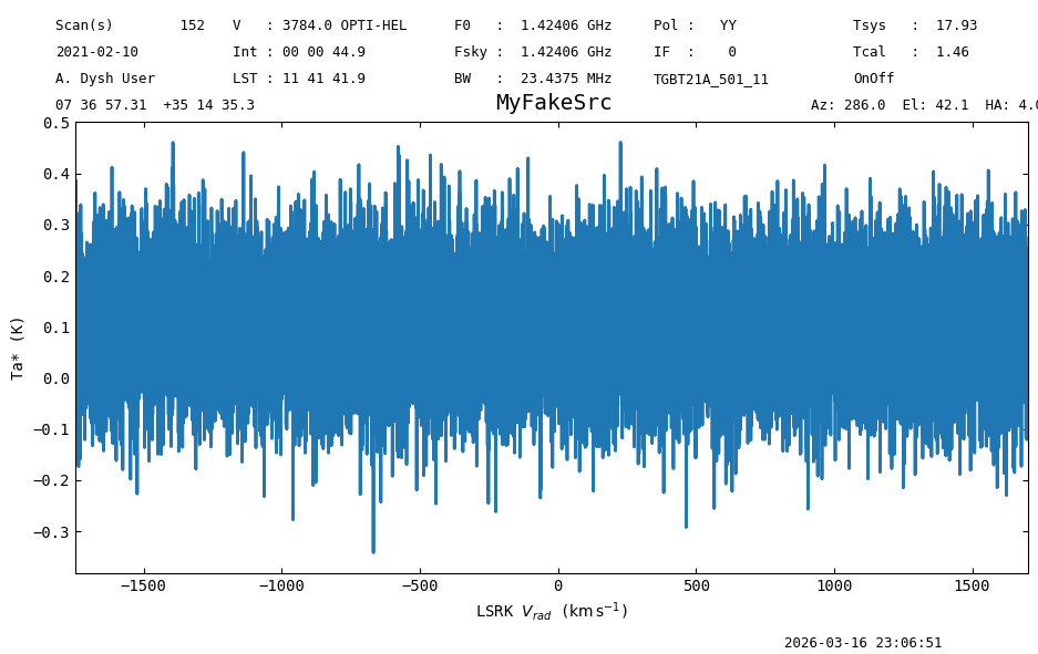
For this example we construct a fake spectrum, with 16384 channels that are 1 kHz wide and a rest frequency of 1.4240575 GHz.

cdelt1 = float((1000*u.Hz).value)
nchan = 16384
restfreq = float((1.4240575*u.GHz).to(u.Hz).value)
crval1 = restfreq
s = Spectrum.fake_spectrum(nchan=nchan, 
                           seed=123,
                           crval1=crval1, 
                           restfrq=restfreq, 
                           freqres=cdelt1, 
                           cdelt1=cdelt1, 
                           obsfreq=restfreq, 
                           dopfreq=restfreq, 
                           object='MyFakeSrc')

print(f"Spectrum redshift is {s.redshift}")

Spectrum redshift is 0.012754329663835273

s.plot(vel_frame='lsrk', doppler_convention='radio', xaxis_unit='km/s');

../_images/214637a96f90a369543a9b17ce5975563ab53de09b79dc71aebd239085af9d0a.png

Find the hydrogen recombination lines that could be in this spectrum, and display their name, chemical name and frequency (in MHz).

s.recomb(line='hydrogen', cat='gbtrecomb', columns=['name', 'chemical_name', 'rest_frequency','obs_frequency'])

Table length=5

name	chemical_name	rest_frequency	obs_frequency

str10	str27	float64	float64
Hγ	Hydrogen Recombination Line	1436.17485014444	1418.0880871880854
Hβ	Hydrogen Recombination Line	1440.71993807134	1422.5759356166463
Hε	Hydrogen Recombination Line	1443.2677438484002	1425.0916550783502
Hδ	Hydrogen Recombination Line	1446.14393752243	1427.9316268165944
Hζ	Hydrogen Recombination Line	1447.12682709455	1428.9021381670088

Find all lines in the spectrum’s frequency range.

s.query_lines(cat='gbtlines',columns=['name', 'chemical_name', 'rest_frequency','obs_frequency'])

Table length=25

name	chemical_name	rest_frequency	obs_frequency

str62	str16	float64	float64
17OH	Hydroxyl radical	1445.0345	1426.8361612234746
ND<sub>3</sub>	Ammonia	1434.448	1416.3829844856236
ND<sub>3</sub>	Ammonia	1434.448	1416.3829844856236
ND<sub>3</sub>	Ammonia	1434.448	1416.3829844856236
ND<sub>3</sub>	Ammonia	1434.448	1416.3829844856236
ND<sub>3</sub>	Ammonia	1437.179	1419.0795910761938
ND<sub>3</sub>	Ammonia	1448.056	1429.819609342628
ND<sub>3</sub>	Ammonia	1448.056	1429.819609342628
ND<sub>3</sub>	Ammonia	1448.056	1429.819609342628
...	...	...	...
D<sub>2</sub><sup>13</sup>CO	Formaldehyde	1440.6321	1422.4892037520992
c-H<sub>2</sub>C<sub>2</sub><sup>13</sup>CO	Cyclopropenone	1440.0488	1421.9132496604552
c-HDC<sub>3</sub>O	Cyclopropenone	1446.9711	1428.7483722536094
<sup>13</sup>CH<sub>2</sub>CHCN	Vinyl Cyanide	1439.3028	1421.1766445646788
CH<sub>3</sub>CH<sub>2</sub>CN <font color="red">v = 0 </font>	Ethyl Cyanide	1437.2031	1419.1033875678936
CH<sub>3</sub>CH<sub>2</sub>CN <font color="red">v = 0 </font>	Ethyl Cyanide	1437.2589	1419.1584848391328
CH<sub>3</sub>CH<sub>2</sub>CN <font color="red">v = 0 </font>	Ethyl Cyanide	1437.4528	1419.349942919657
CH<sub>2</sub>CN	Cyanomethyl	1439.976	1421.841366482208
<sup>13</sup>CH<sub>2</sub>CHCN	Vinyl Cyanide	1439.3028	1421.1766445646788

To clear the cache, use:

SpectralLineSearch.clear_cache()

Final Stats#

Finally, at the end we compute some statistics over a spectrum, merely as a checksum if the notebook is reproducible.

s.check_stats(0.09961288 * u.K)

23:06:52.481 I rms is OK