Selecting Data

Selecting Data#

This notebook shows how to select data in dysh. By selecting data, you can narrow down which scans or integrations the subsequent calibration routines will operate on. We call such narrowing down a “selection rule.” You create selection rules through methods of GBTFITSLoad, which uses an instance of Selection as an attribute called selection. You can create multiple selection rules that will be logically ANDed to create a final rule at calibration time.

Dysh commands#

The following dysh commands are introduced (leaving out all the function arguments):

  filename = dysh_data()
  sdf = GBTFITSLoad()
  sdf.select()
  sb = sdf.getps()
  ta = sb.timeaverage()
  ta.baseline()
  ta.average()
  ta.plot()
  ta_plt.savefig()

Loading Modules#

We start by loading the modules we will use in this notebook.

# These modules are required for the notebook (no plotting is done)
import astropy.units as u
from astropy.time import Time
from dysh.log import init_logging
from dysh.fits.gbtfitsload import GBTFITSLoad
from dysh.log import init_logging

# These modules are used for file I/O
from dysh.util.files import dysh_data
from pathlib import Path

Setup#

We start the dysh logging, so we get more information about what is happening. This is only needed if working on a notebook. If using the CLI through the dysh command, then logging is setup for you.

init_logging(2)

# also create a local "output" directory where temporary notebook files can be stored.
output_dir = Path.cwd() / "output"
output_dir.mkdir(exist_ok=True)

Data Retrieval#

Download the example SDFITS data, if necessary.

The code below will download an SDFITS file from and put it in a data directory.

The code below will download an SDFITS file from http://www.gb.nrao.edu/dysh/example_data and put it in a data directory. The data directory must exist where this notebook is being run from, otherwise the downloaded SDFITS will be named data. The example will work either way, but be aware if you find a new file named data after running it.

# hi-survey/data/AGBT04A_008_02.raw.acs/AGBT04A_008_02.raw.acs.fits
filename = dysh_data(example="survey")

23:08:39.822 I Resolving example=survey -> hi-survey/data/AGBT04A_008_02.raw.acs/AGBT04A_008_02.raw.acs.fits

23:08:39.823 I url: http://www.gb.nrao.edu/dysh//example_data/hi-survey/data/AGBT04A_008_02.raw.acs/AGBT04A_008_02.raw.acs.fits

AGBT04A_008_02.raw.acs.fits already downloaded

Data Loading#

Next, we use GBTFITSLoad to load the data, and then its summary method to inspect its contents. We add the UTC column to the summary.

sdfits = GBTFITSLoad(filename)
sdfits.summary(add_columns=["UTC"])

SCAN	OBJECT	VELOCITY	PROC	PROCSEQN	RESTFREQ	# IF	# POL	# INT	# FEED	AZIMUTH	ELEVATION	UTC
220	3C286	0.0	OffOn	1	1.400000	1	2	6	1	185.2806	82.0246	2004-04-22 04:51:41.035000192
221	3C286	0.0	OffOn	2	1.400000	1	2	6	1	187.2136	81.9980	2004-04-22 04:52:56.034999936
222	3C286	0.0	OffOn	1	1.400000	1	2	6	1	193.8331	81.8413	2004-04-22 04:57:18.034999936
223	3C286	0.0	OffOn	2	1.400000	1	2	6	1	195.6766	81.7788	2004-04-22 04:58:33.035000192
224	3C286	0.0	OffOn	1	1.400000	1	2	6	1	195.5182	80.2910	2004-04-22 05:00:06.034999936
225	3C286	0.0	OffOn	2	1.400000	1	2	5	1	199.9358	81.6005	2004-04-22 05:01:31.028000128
226	3C286	0.0	OffOn	1	1.400000	1	2	6	1	200.8333	80.0265	2004-04-22 05:04:25.035000192
227	3C286	0.0	OffOn	2	1.400000	1	2	6	1	205.9471	81.2609	2004-04-22 05:05:57.035000192
228	B1328+254	0.0	OffOn	1	1.400000	1	2	6	1	207.5257	73.9844	2004-04-22 05:17:26.034999936
229	B1328+254	0.0	OffOn	2	1.400000	1	2	6	1	210.9600	75.1584	2004-04-22 05:18:54.034999936
230	B1345+125	0.0	OffOn	1	1.400000	1	2	18	1	193.2738	62.0703	2004-04-22 05:27:20.118333440
231	B1345+125	0.0	OffOn	2	1.400000	1	2	18	1	195.6794	63.3244	2004-04-22 05:30:43.118333440
244	B1345+125	0.0	OffOn	1	1.400000	1	2	18	1	200.9543	60.9284	2004-04-22 05:45:21.118333440
245	B1345+125	0.0	OffOn	2	1.400000	1	2	18	1	203.5311	62.0587	2004-04-22 05:48:43.118333440
246	B1345+125	0.0	OffOn	1	1.400000	1	2	18	1	204.3408	60.3930	2004-04-22 05:52:26.006111104
247	B1345+125	0.0	OffOn	2	1.400000	1	2	18	1	206.9763	61.4655	2004-04-22 05:55:48.006111232
248	B1345+125	0.0	OffOn	1	1.370000	1	2	18	1	208.0408	59.6983	2004-04-22 06:00:27.118333440
249	B1345+125	0.0	OffOn	2	1.370000	1	2	18	1	210.7215	60.7060	2004-04-22 06:03:49.118333440
250	B1345+125	0.0	Track	1	1.370000	1	2	3	1	215.2430	59.6119	2004-04-22 06:08:15.013333504
251	B1345+125	0.0	Track	1	1.370000	1	2	3	1	215.9692	59.4175	2004-04-22 06:09:57.013333120
263	U8091	213.0	OffOn	1	1.420405	1	2	30	1	241.1339	50.6393	2004-04-22 06:31:44.201666816
264	U8091	213.0	OffOn	2	1.420405	1	2	30	1	240.9795	50.7395	2004-04-22 06:37:07.201666688
265	U8091	213.0	Track	1	1.420405	1	2	3	1	243.4807	49.8234	2004-04-22 06:40:42.013332992
266	U8249	2541.0	OffOn	1	1.420405	1	2	10	1	241.7065	50.2801	2004-04-22 06:45:34.062999936
267	U8249	2541.0	OffOn	1	1.420405	1	2	30	1	242.6892	49.6343	2004-04-22 06:49:17.011333376
268	U8249	2541.0	OffOn	2	1.420405	1	2	30	1	242.5451	49.7333	2004-04-22 06:54:41.011333248
269	U8249	2541.0	Track	1	1.420405	1	2	3	1	244.9435	48.0787	2004-04-22 06:58:18.013332992
270	U8503	4676.0	OffOn	1	1.420405	1	2	30	1	270.1741	60.2485	2004-04-22 07:05:18.201666816
271	U8503	4676.0	OffOn	2	1.420405	1	2	30	1	269.9396	60.5449	2004-04-22 07:10:40.201666816
272	U8091	213.0	OffOn	1	1.420405	1	2	30	1	253.5780	41.4420	2004-04-22 07:21:01.011333376
273	U8091	213.0	OffOn	2	1.420405	1	2	30	1	253.4586	41.5517	2004-04-22 07:26:24.011333632
274	U8091	213.0	Track	1	1.420405	1	2	3	1	255.5793	39.5541	2004-04-22 07:31:11.013333504
275	U8249	2541.0	OffOn	1	1.420405	1	2	30	1	266.5469	46.8377	2004-04-22 07:36:10.011333376
276	U8249	2541.0	OffOn	2	1.420405	1	2	30	1	266.3738	47.0388	2004-04-22 07:41:31.011333376
277	U8249	2541.0	Track	1	1.420405	1	2	3	1	267.9426	45.1863	2004-04-22 07:45:11.013333504
278	U9965	4524.0	OffOn	1	1.420405	1	2	30	1	221.5582	67.7182	2004-04-22 07:52:57.011333248
279	U9965	4524.0	OffOn	2	1.420405	1	2	30	1	221.2070	67.8070	2004-04-22 07:58:27.011333632
280	U9965	4524.0	Track	1	1.420405	1	2	3	1	222.9262	67.3657	2004-04-22 08:01:49.013333120
281	U10351	891.0	OffOn	1	1.420405	1	2	30	1	221.2955	77.4668	2004-04-22 08:09:01.011333376
282	U10351	891.0	OffOn	2	1.420405	1	2	30	1	220.4924	77.5922	2004-04-22 08:14:38.011333248
283	U10351	891.0	Track	1	1.420405	1	2	3	1	227.9032	76.2644	2004-04-22 08:18:33.013333120
284	U9007	4618.0	OffOn	1	1.420405	1	2	30	1	248.6632	38.3497	2004-04-22 08:26:53.011333376
285	U9007	4618.0	OffOn	2	1.420405	1	2	30	1	248.5549	38.4433	2004-04-22 08:32:14.011333248
286	U9007	4618.0	Track	1	1.420405	1	2	3	1	250.5574	36.6787	2004-04-22 08:36:03.013333504
287	U9007	5257.0	OffOn	1	1.420405	1	2	30	1	234.2956	48.0209	2004-04-22 08:41:26.011333248
288	U9007	5257.0	OffOn	2	1.420405	1	2	30	1	234.1669	48.0937	2004-04-22 08:46:50.011333376
289	U9803	5257.0	OffOn	1	1.420405	1	2	30	1	264.9610	57.9997	2004-04-22 08:56:18.011333120
290	U9803	5257.0	OffOn	2	1.420405	1	2	30	1	264.7276	58.2483	2004-04-22 09:01:40.011333504
291	U9803	5257.0	Track	1	1.420405	1	2	3	1	266.5221	56.2884	2004-04-22 09:05:54.013332992
292	U10351	891.0	OffOn	1	1.420405	1	2	30	1	252.1644	67.0847	2004-04-22 09:11:13.011333248
293	U10351	891.0	OffOn	2	1.420405	1	2	30	1	251.8134	67.3038	2004-04-22 09:16:38.011333248
294	U10351	891.0	Track	1	1.420405	1	2	3	1	255.3764	64.9184	2004-04-22 09:23:31.013333504
295	U10629	2980.0	OffOn	1	1.420405	1	2	30	1	233.9472	66.8551	2004-04-22 09:29:00.011333248
296	U10629	2980.0	OffOn	2	1.420405	1	2	30	1	233.5991	66.9846	2004-04-22 09:34:28.011333504
297	U10629	2980.0	OffOn	1	1.420405	1	2	30	1	238.3584	65.0614	2004-04-22 09:40:00.011333632
298	U10629	2980.0	OffOn	2	1.420405	1	2	30	1	238.0441	65.2006	2004-04-22 09:45:27.011333504
299	U10629	2980.0	Track	1	1.420405	1	2	3	1	241.4405	63.6131	2004-04-22 09:49:02.013332992
300	U11017	4644.0	OffOn	1	1.420405	1	2	30	1	235.4605	76.2074	2004-04-22 09:54:06.011333248
301	U11017	4644.0	OffOn	2	1.420405	1	2	30	1	234.7726	76.3879	2004-04-22 09:59:39.011333376
302	U11017	4644.0	OffOn	1	1.420405	1	2	30	1	241.5197	74.3514	2004-04-22 10:05:11.011333504
303	U11017	4644.0	OffOn	2	1.420405	1	2	30	1	240.9590	74.5471	2004-04-22 10:10:43.011333632
304	U11017	4644.0	Track	1	1.420405	1	2	3	1	242.6641	73.9425	2004-04-22 10:14:13.013333120
305	U11017	4644.0	Track	1	1.420405	1	2	1	1	242.9359	73.8408	2004-04-22 10:14:48
306	U11017	4644.0	Track	1	1.420405	1	2	3	1	246.0511	72.5738	2004-04-22 10:16:10.013332992
307	U11461	3122.0	OffOn	1	1.420405	1	2	30	1	168.0531	59.8975	2004-04-22 10:25:22.011333120
308	U11461	3122.0	OffOn	2	1.420405	1	2	30	1	167.8894	59.8843	2004-04-22 10:30:53.011333376
309	U11461	3122.0	OffOn	1	1.420405	1	2	30	1	173.4698	60.2443	2004-04-22 10:36:22.011333248
310	U11461	3122.0	OffOn	2	1.420405	1	2	30	1	173.3111	60.2376	2004-04-22 10:41:54.011333120
311	U11461	3122.0	Track	1	1.420405	1	2	3	1	178.1207	60.3802	2004-04-22 10:45:45.013333120
312	U11578	4601.0	OffOn	1	1.420405	1	2	30	1	156.3573	58.8036	2004-04-22 10:52:22.011333248
313	U11578	4601.0	OffOn	2	1.420405	1	2	30	1	156.1796	58.7731	2004-04-22 10:57:50.011333248
314	U11578	4601.0	Track	1	1.420405	1	2	3	1	160.4469	59.4464	2004-04-22 11:01:18.999999872
315	U11578	4601.0	Track	1	1.420405	1	2	3	1	161.0040	59.5231	2004-04-22 11:02:30.013332992
316	U11627	4864.0	OffOn	1	1.420405	1	2	30	1	157.8065	55.3372	2004-04-22 11:07:12.011333632
317	U11627	4864.0	OffOn	2	1.420405	1	2	30	1	157.6549	55.3107	2004-04-22 11:12:39.011333504
318	U11627	4864.0	OffOn	1	1.420405	1	2	30	1	162.4625	56.0655	2004-04-22 11:18:07.011333248
319	U11627	4864.0	OffOn	2	1.420405	1	2	30	1	162.3199	56.0465	2004-04-22 11:23:36.011333376
320	U11627	4864.0	Track	1	1.420405	1	2	3	1	166.7983	56.5802	2004-04-22 11:28:00.013333376
321	U11992	3592.0	Track	1	1.420405	1	2	3	1	124.4762	54.3242	2004-04-22 11:32:01.013333120
322	U11992	3592.0	OffOn	1	1.420405	1	2	30	1	125.6320	54.9128	2004-04-22 11:35:30.011333120
323	U11992	3592.0	OffOn	2	1.420405	1	2	30	1	125.4565	54.8251	2004-04-22 11:40:55.011333504

Using Selection#

Now we show various ways in which GBTFITSLoad.selection can be used to select data.

Select by column value#

One way of selecting data is by specifying a value for an SDFITS column name. (The column name case insensitive, but the value is not). For example, we can select data which has OBJECT=”U8249” or OBJECT=”U8249” using the following.

Note Selecting values in a list will logically OR those values. So object=["U8249","U11017"] will select scans with either object. But multiple keywords (columns) will be logically ANDed (see below).

sdfits.select(object=["U8249","U11017"])

We can view the contents of the selection using its show method. This displays the selection as a table. The # Selected column gives the number of records (integrations) selected by each selection rule. Each time we create a new selection, it is assigned a unique id and tag.

sdfits.selection.show()

 ID    TAG          OBJECT       # SELECTED
--- --------- ------------------ ----------
  0 919e9c43a ['U8249','U11017']        572

We can also specify the tag name to have a more meaningful value.

sdfits.select(proc="OffOn", tag='proc onoff')

sdfits.selection.show()

 ID    TAG           OBJECT        PROC # SELECTED
--- ---------- ------------------ ----- ----------
  0  919e9c43a ['U8249','U11017']              572
  1 proc onoff                    OffOn       3540

Combining Selections#

Once we have multiple selection rules in the Selection object, we can combine them into a single selection using the final property. This will return a pandas.DataFrame.

sdfits.selection.final

	OBJECT	BANDWID	DATE-OBS	DURATION	EXPOSURE	TSYS	TDIM7	TUNIT7	CTYPE1	CRVAL1	...	SITELAT	SITEELEV	EXTNAME	FITSINDEX	UTC	CHAN	PROC	OBSTYPE	SUBOBSMODE	INTNUM
0	U8249	12500000.0	2004-04-22T06:44:49.00	5.005	4.779488	1.0	(32768,1,1,1)	Counts	FREQ-OBS	1.408421e+09	...	38.43312	824.595	SINGLE DISH	0	2004-04-22 06:44:49.000	None	OffOn	PSWITCHOFF	TPWCAL	0
1	U8249	12500000.0	2004-04-22T06:44:49.00	5.005	4.779488	1.0	(32768,1,1,1)	Counts	FREQ-OBS	1.408421e+09	...	38.43312	824.595	SINGLE DISH	0	2004-04-22 06:44:49.000	None	OffOn	PSWITCHOFF	TPWCAL	0
2	U8249	12500000.0	2004-04-22T06:44:49.00	5.005	4.779488	1.0	(32768,1,1,1)	Counts	FREQ-OBS	1.408421e+09	...	38.43312	824.595	SINGLE DISH	0	2004-04-22 06:44:49.000	None	OffOn	PSWITCHOFF	TPWCAL	0
3	U8249	12500000.0	2004-04-22T06:44:49.00	5.005	4.779488	1.0	(32768,1,1,1)	Counts	FREQ-OBS	1.408421e+09	...	38.43312	824.595	SINGLE DISH	0	2004-04-22 06:44:49.000	None	OffOn	PSWITCHOFF	TPWCAL	0
4	U8249	12500000.0	2004-04-22T06:44:59.01	5.005	4.779488	1.0	(32768,1,1,1)	Counts	FREQ-OBS	1.408421e+09	...	38.43312	824.595	SINGLE DISH	0	2004-04-22 06:44:59.010	None	OffOn	PSWITCHOFF	TPWCAL	1
...	...	...	...	...	...	...	...	...	...	...	...	...	...	...	...	...	...	...	...	...	...
515	U11017	12500000.0	2004-04-22T10:12:48.02	10.000	9.596709	1.0	(32768,1,1,1)	Counts	FREQ-OBS	1.398806e+09	...	38.43312	824.595	SINGLE DISH	0	2004-04-22 10:12:48.020	None	OffOn	PSWITCHON	TPNOCAL	27
516	U11017	12500000.0	2004-04-22T10:12:58.02	10.000	9.596709	1.0	(32768,1,1,1)	Counts	FREQ-OBS	1.398806e+09	...	38.43312	824.595	SINGLE DISH	0	2004-04-22 10:12:58.020	None	OffOn	PSWITCHON	TPNOCAL	28
517	U11017	12500000.0	2004-04-22T10:12:58.02	10.000	9.596709	1.0	(32768,1,1,1)	Counts	FREQ-OBS	1.398806e+09	...	38.43312	824.595	SINGLE DISH	0	2004-04-22 10:12:58.020	None	OffOn	PSWITCHON	TPNOCAL	28
518	U11017	12500000.0	2004-04-22T10:13:08.02	10.000	9.596709	1.0	(32768,1,1,1)	Counts	FREQ-OBS	1.398806e+09	...	38.43312	824.595	SINGLE DISH	0	2004-04-22 10:13:08.020	None	OffOn	PSWITCHON	TPNOCAL	29
519	U11017	12500000.0	2004-04-22T10:13:08.02	10.000	9.596709	1.0	(32768,1,1,1)	Counts	FREQ-OBS	1.398806e+09	...	38.43312	824.595	SINGLE DISH	0	2004-04-22 10:13:08.020	None	OffOn	PSWITCHON	TPNOCAL	29

520 rows × 94 columns

In this particular case, we wind up with 520 integrations. This is a selection of objects U8249 or U11017 AND proc OnOff. Because keywords in the same selection rule are logically ANDed, this could also have been accomplished via

sdfits.select(object=["U8249","U11017"], proc="OffOn")

(Try it yourself).

You can also see a summary of the selected data, using the selected argument of summary:

sdfits.summary(selected=True)

SCAN	OBJECT	VELOCITY	PROC	PROCSEQN	RESTFREQ	# IF	# POL	# INT	# FEED	AZIMUTH	ELEVATION
266	U8249	2541.0	OffOn	1	1.420405	1	2	10	1	241.7065	50.2801
267	U8249	2541.0	OffOn	1	1.420405	1	2	30	1	242.6892	49.6343
268	U8249	2541.0	OffOn	2	1.420405	1	2	30	1	242.5451	49.7333
275	U8249	2541.0	OffOn	1	1.420405	1	2	30	1	266.5469	46.8377
276	U8249	2541.0	OffOn	2	1.420405	1	2	30	1	266.3738	47.0388
300	U11017	4644.0	OffOn	1	1.420405	1	2	30	1	235.4605	76.2074
301	U11017	4644.0	OffOn	2	1.420405	1	2	30	1	234.7726	76.3879
302	U11017	4644.0	OffOn	1	1.420405	1	2	30	1	241.5197	74.3514
303	U11017	4644.0	OffOn	2	1.420405	1	2	30	1	240.9590	74.5471

Remove selection rules#

You can remove a selection rule by id or tag. Multiple rows with the same tag will all be removed.

sdfits.selection.remove(id=0)
sdfits.selection.show()

 ID    TAG      PROC # SELECTED
--- ---------- ----- ----------
  1 proc onoff OffOn       3540

To remove all selection rules use clear_selection. After using it, the Selection will show no selection rules.

sdfits.clear_selection()
sdfits.selection.show()

 ID TAG OBJECT BANDWID DATE-OBS ... SUBOBSMODE FITSINDEX CHAN UTC # SELECTED
--- --- ------ ------- -------- ... ---------- --------- ---- --- ----------

Select by Range#

It is also possible to define a selection given a range of values using select_range. In this case the selection must be specified using either a list, [], or a tuple, (), with a start and an end value. Ranges are considered inclusive of both ends. Lower limits are give by (value,None) or (value,). Upper limits are given by (None,value), since (,value) is not valid Python. For coordinates the default unit is taken to be degrees. Other units can be explicitly given. Both () and [] are valid for indicated ranges, but only tuples can be a lower limit (value,).

For example to select only rows where the right ascension is greater than 114 degrees:

sdfits.select_range(ra=(114,), tag="RA>=114 deg")
sdfits.selection.show()

 ID     TAG            CRVAL2       # SELECTED
--- ----------- ------------------- ----------
  0 RA>=114 deg [np.float64(114.0)]       3766

(Right Ascension is the FITS CRVAL2 column).

To select rows where the elevation is below 80 degrees:

sdfits.select_range(elevation=[None,80], tag="EL<80")
sdfits.selection.show()

 ID     TAG            CRVAL2        ELEVATIO # SELECTED
--- ----------- ------------------- --------- ----------
  0 RA>=114 deg [np.float64(114.0)]                 3766
  1       EL<80                     [None,80]       3582

(Note elevation column is ELEVATIO because the FITS standard only allow 8 characters for column names).

We can check that the selections were applied properly by inspecting the final result and a subset of its columns.

sdfits.selection.final[["OBJECT","CRVAL2","ELEVATIO"]]

	OBJECT	CRVAL2	ELEVATIO
0	3C286	202.784508	79.997019
1	3C286	202.784508	79.997019
2	3C286	202.784508	79.997019
3	3C286	202.784508	79.997019
4	B1328+254	202.066324	74.023075
...	...	...	...
3577	U11992	335.197517	55.157387
3578	U11992	335.197520	55.183819
3579	U11992	335.197520	55.183819
3580	U11992	335.197546	55.210211
3581	U11992	335.197546	55.210211

3582 rows × 3 columns

It is also possible to use units during selection. For example

sdfits.select_range(dec=[854, 855] * u.arcmin, tag="14.23<=DEC<=14.25")
sdfits.selection.show()

 ID        TAG               CRVAL2       ...  ELEVATIO # SELECTED
--- ----------------- ------------------- ... --------- ----------
  0       RA>=114 deg [np.float64(114.0)] ...                 3766
  1             EL<80                     ... [None,80]       3582
  2 14.23<=DEC<=14.25                     ...                  132

sdfits.summary(selected=True)

SCAN	OBJECT	VELOCITY	PROC	PROCSEQN	RESTFREQ	# IF	# POL	# INT	# FEED	AZIMUTH	ELEVATION
321	U11992	3592.0	Track	1	1.420405	1	2	3	1	124.4762	54.3242
322	U11992	3592.0	OffOn	1	1.420405	1	2	30	1	125.6320	54.9128
323	U11992	3592.0	OffOn	2	1.420405	1	2	30	1	125.4565	54.8251

Select Within a Range#

It is also possible to specify the midpoint and a range to make a selection. In this case we use select_within and specify the mean value and the +- range.

For example to select between elevation of 50-10 and 50+10 we would use

sdfits.select_within(elevation=(50,10), tag="EL=50+/-10")
sdfits.selection.show()

 ID        TAG               CRVAL2       ...  ELEVATIO # SELECTED
--- ----------------- ------------------- ... --------- ----------
  0       RA>=114 deg [np.float64(114.0)] ...                 3766
  1             EL<80                     ... [None,80]       3582
  2 14.23<=DEC<=14.25                     ...                  132
  3        EL=50+/-10                     ...   [40,60]       1694

Which shows a selection between 40 and 60 degrees of elevation.

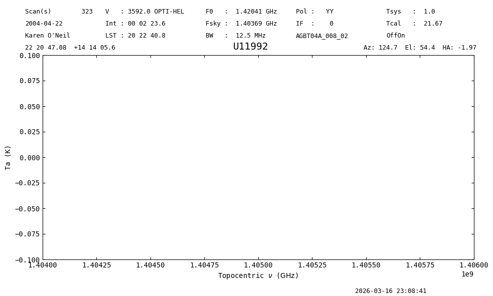
Now, when you do a getps it will operate only on the selected data.

(Currently, you can’t preselect ifnum, plnum, or fdnum; they must be provided as method arguments).

sb = sdfits.getps(ifnum=0, plnum=0, fdnum=0)
sb.timeaverage().plot(ymin=-.1, ymax=.1, xmin=1.404E9, xmax=1.406E9);

23:08:41.078 I Using TSYS column

../_images/1cc401f5c19cb52e0a34e71fd785f3c55859d98a515621d9e57aa01805bb286e.png

Using Aliases#

Selection knows about certain aliases for column names. For example, the SDFITS column ELEVATIO can also be selected using ELEVATION. The aliases are defined in the aliases attribute of Selection.

sdfits.selection.aliases

{'FREQ': 'CRVAL1',
 'RA': 'CRVAL2',
 'DEC': 'CRVAL3',
 'GLON': 'CRVAL2',
 'GLAT': 'CRVAL3',
 'GALLON': 'CRVAL2',
 'GALLAT': 'CRVAL3',
 'ELEVATION': 'ELEVATIO',
 'SOURCE': 'OBJECT',
 'POL': 'PLNUM',
 'SUBREF': 'SUBREF_STATE'}

It is also possible to add your own aliases. For example to use target and az as aliases for OBJECT and AZIMUTH we would use

sdfits.selection.alias({'target':'object','az':'azimuth'})
sdfits.selection.aliases

{'FREQ': 'CRVAL1',
 'RA': 'CRVAL2',
 'DEC': 'CRVAL3',
 'GLON': 'CRVAL2',
 'GLAT': 'CRVAL3',
 'GALLON': 'CRVAL2',
 'GALLAT': 'CRVAL3',
 'ELEVATION': 'ELEVATIO',
 'SOURCE': 'OBJECT',
 'POL': 'PLNUM',
 'SUBREF': 'SUBREF_STATE',
 'TARGET': 'OBJECT',
 'AZ': 'AZIMUTH'}

Then you can select using your aliases:

sdfits.select(target="U8249")
sdfits.selection.show()

 ID        TAG        OBJECT ...  ELEVATIO # SELECTED
--- ----------------- ------ ... --------- ----------
     RA>=114 deg        ...                 3766
           EL<80        ... [None,80]       3582
14.23<=DEC<=14.25        ...                  132
      EL=50+/-10        ...   [40,60]       1694
       cfffdc371  U8249 ...                  304

Notice that this will only affect the aliases for this particular instance of a GBTFITSLoad. Any new GBTFITSLoad objects will not know about these aliases.

Empty Selections#

Any selection that results in no data being selected is ignored. You will get a warning message in this case.

sdfits.selection.select(target='foobar')
sdfits.selection.show()

23:08:42.503 W Your selection rule resulted in no data being selected. Ignoring.

 ID        TAG        OBJECT ...  ELEVATIO # SELECTED
--- ----------------- ------ ... --------- ----------
     RA>=114 deg        ...                 3766
           EL<80        ... [None,80]       3582
14.23<=DEC<=14.25        ...                  132
      EL=50+/-10        ...   [40,60]       1694
       cfffdc371  U8249 ...                  304

Time Selections#

UTC time ranges can be selected with astropy.time.Time objects. This checks against the UTC timestamp column. For LST, use select_range(lst=[number1,number2]).

# clear the selection for this demonstration
sdfits.clear_selection()

sdfits.select_range(utc=(Time("2004-04-22T05:27:20.12", scale="utc"),
                         Time("2004-04-22T05:48:43.12", scale="utc")),
                    tag="time range")
sdfits.selection.show()

 ID    TAG     ... # SELECTED
--- ---------- ... ----------
  0 time range ...        216

sdfits.selection.final[["SCAN","OBJECT","UTC", "LST","PLNUM","IFNUM","FDNUM"]]

	SCAN	OBJECT	UTC	LST	PLNUM	IFNUM	FDNUM
0	230	B1345+125	2004-04-22 05:27:25.130	51035.015413	1	0	0
1	230	B1345+125	2004-04-22 05:27:25.130	51035.015413	1	0	0
2	230	B1345+125	2004-04-22 05:27:25.130	51035.015413	0	0	0
3	230	B1345+125	2004-04-22 05:27:25.130	51035.015413	0	0	0
4	230	B1345+125	2004-04-22 05:27:35.140	51045.056730	1	0	0
...	...	...	...	...	...	...	...
211	245	B1345+125	2004-04-22 05:48:28.100	52301.445514	0	0	0
212	245	B1345+125	2004-04-22 05:48:38.110	52311.486833	1	0	0
213	245	B1345+125	2004-04-22 05:48:38.110	52311.486833	1	0	0
214	245	B1345+125	2004-04-22 05:48:38.110	52311.486833	0	0	0
215	245	B1345+125	2004-04-22 05:48:38.110	52311.486833	0	0	0

216 rows × 7 columns

Channel Selection#

You can selection a contiguous range of channels using select_channel, and the integrations will be trimmed to that channel range during calibration. The final spectrum will have the input channel range. As with select_range, channel ranges are inclusive at both ends.

sdfits.select_channel([2000,6000], tag="channels")

sdfits.selection.show()

 ID    TAG     ... # SELECTED
--- ---------- ... ----------
  0 time range ...        216
  1   channels ...       3766

sb = sdfits.getps(ifnum=0, plnum=1, fdnum=0)
sb.timeaverage().plot(xaxis_unit="channel");

23:08:42.761 I Ignoring 9 blanked integration(s).

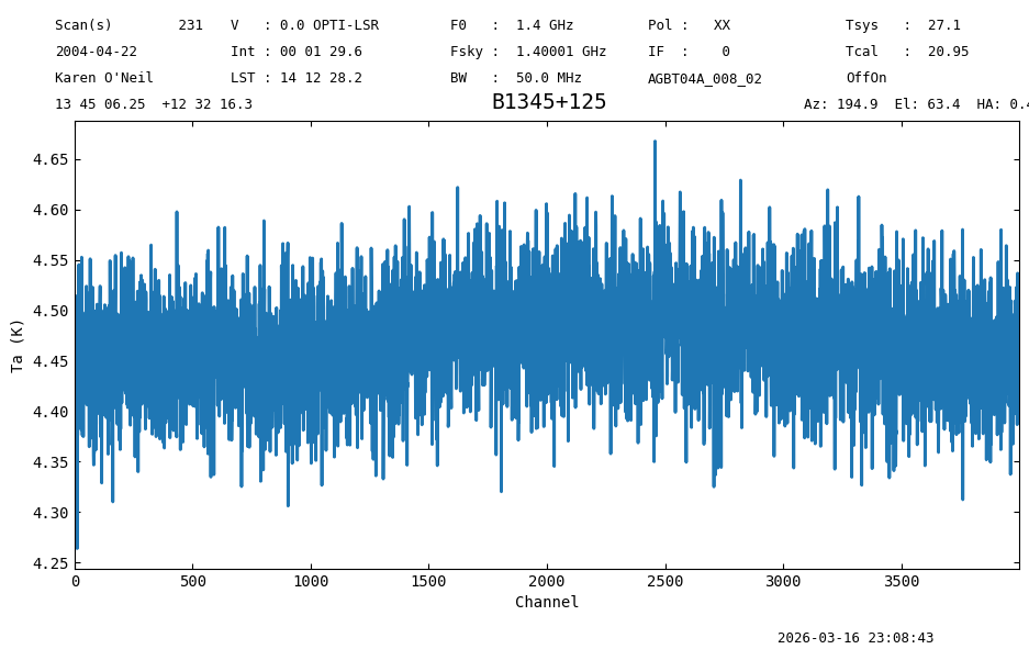
../_images/4c42f5462b4c4fb1f69985d8182c4160fb96a559dfc53cb3a94b594c139dbd44.png

The resulting Spectrum only has 4000 channels, as specified by the channel selection.

Note that you can only have one channel selection rule at a time.

try: 
    sdfits.select_channel([60,70])
except Exception as e:
    print(e)

You can only have one channel selection rule. Remove the old rule before creating a new one.

Final Stats#

Finally, at the end we compute some statistics over a spectrum, merely as a checksum if the notebook is reproducible.

This particular case has a mixed number of scanblocks, so we just pick the first.

sb.timeaverage().check_stats(0.05038713 * u.K)

23:08:43.435 I rms is OK