Smoothing

This notebook shows how to use dysh to smooth a spectrum.

For the example below we will use data from the Position-Switch example again. The following dysh commands are the simplest to get and smooth a spectrum (leaving out all the function arguments):

  sdf = GBTFITSLoad()
  sb = sdf.getps()
  ta = sb.timeaverage()
  tb = ta.smooth()
  tb.plot()

or if you wish to make use of the Python object chaining you can do this in one line:

   GBTFITSLoad().getps().timeaverage().smooth().plot()

Loading Modules

We start by loading the modules we will use for the data reduction.

# These modules are required for working with the data.
from dysh.fits.gbtfitsload import GBTFITSLoad
from dysh.log import init_logging
from astropy import units as u

# These modules are used for file I/O
from dysh.util.files import dysh_data
from pathlib import Path

Setup

We start the dysh logging, so we get more information about what is happening. This is only needed if working on a notebook. If using the CLI through the dysh command, then logging is setup for you.

init_logging(2)

# also create a local "output" directory where temporary notebook files can be stored.
output_dir = Path.cwd() / "output"
output_dir.mkdir(exist_ok=True)

Data Retrieval

Download the example SDFITS data, if necessary.

filename = dysh_data(test="getps")

23:08:47.000 I Resolving test=getps -> AGBT05B_047_01/AGBT05B_047_01.raw.acs/

Data Loading

Next, we use GBTFITSLoad to load the data, and then its summary method to inspect its contents.

sdfits = GBTFITSLoad(filename)

23:08:47.052 I Index loaded from .index file (44/93 columns). Missing columns (TCAL, WCS, calibration metadata, etc.) will be automatically loaded from FITS file when first accessed.

sdfits.summary()

SCAN	OBJECT	VELOCITY	PROC	PROCSEQN	RESTFREQ	# IF	# POL	# INT	# FEED	AZIMUTH	ELEVATION
51	NGC5291	4386.0	OnOff	1	1.420405	1	2	11	1	198.3431	18.6427
52	NGC5291	4386.0	OnOff	2	1.420405	1	2	11	1	198.9306	18.7872
53	NGC5291	4386.0	OnOff	1	1.420405	1	2	11	1	199.3305	18.3561
54	NGC5291	4386.0	OnOff	2	1.420405	1	2	11	1	199.9157	18.4927
55	NGC5291	4386.0	OnOff	1	1.420405	1	2	11	1	200.3042	18.0575
56	NGC5291	4386.0	OnOff	2	1.420405	1	2	11	1	200.8906	18.1860
57	NGC5291	4386.0	OnOff	1	1.420405	1	2	11	1	202.3275	17.3853
58	NGC5291	4386.0	OnOff	2	1.420405	1	2	11	1	202.9192	17.4949

Data Reduction

Calibration and Time Averaging

This test data has 8 scans making up 4 pairs of OnOff observations. We will calibrate all of the OnOff scan pairs, time average them and then compare the results with and without smoothing. To calibrate all of the scans, we can omit the scan= keyword when using the sdfits.getps method.

Technical note: getps returns a ScanBlock with in this case four PSScans, since there are four pairs of OnOff observations.

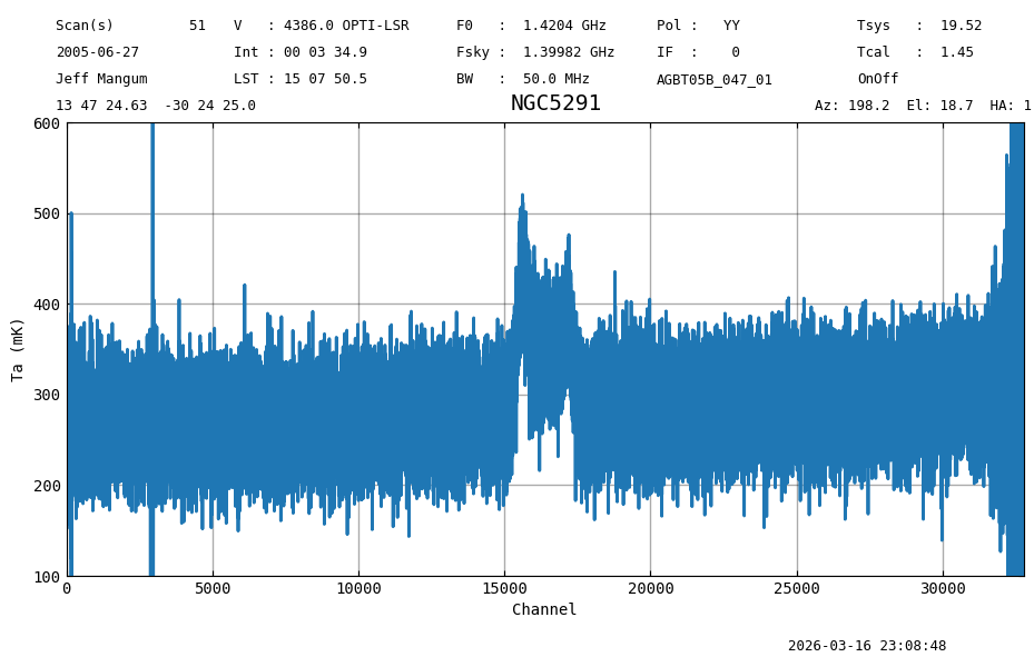
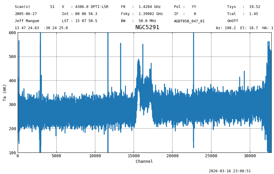
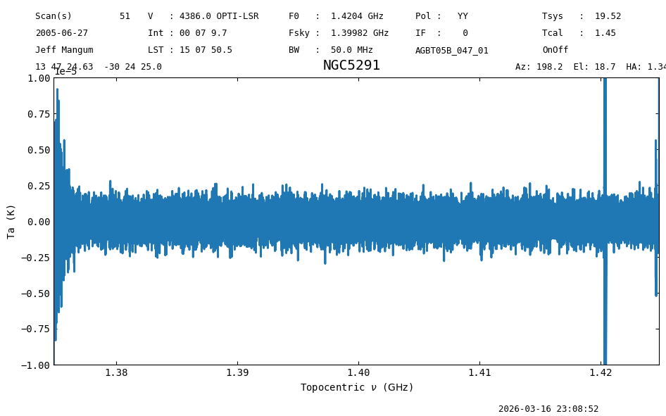
The noise in the time averaged spectrum is 36 mK. However, this has not been baseline subtracted and there is a slope in the continuum. In addition, the edges look horrible, and there is a strong “spike” (galactic) emission near channel 3000. We like to avoid using those data for the baseline fit.

scan_block = sdfits.getps(ifnum=0, plnum=0, fdnum=0)
ta = scan_block.timeaverage()
ta.plot(xaxis_unit="chan", yaxis_unit="mK", ymin=100, ymax=600, grid=True)

# Define a string for printing the spectrum statistics.
fmt_str = "mean: {mean:.4f} median: {median:.4f} rms: {rms:.4f} min: {min:.2f} max: {max:.2f}"
print(f"Stats : {fmt_str}".format(**ta[5000:14000].stats()))
print("Expect: mean: 0.2708 K median: 0.2711 K rms: 0.0359 K min: 0.14 K max: 0.42 K")
print(f"Stats : {fmt_str}".format(**ta[20000:30000].stats()))
print("Expect: mean: 0.2916 K median: 0.2916 K rms: 0.0366 K min: 0.14 K max: 0.41 K")

Stats : mean: 0.2708 K median: 0.2711 K rms: 0.0359 K min: 0.14 K max: 0.42 K
Expect: mean: 0.2708 K median: 0.2711 K rms: 0.0359 K min: 0.14 K max: 0.42 K
Stats : mean: 0.2916 K median: 0.2916 K rms: 0.0366 K min: 0.14 K max: 0.41 K
Expect: mean: 0.2916 K median: 0.2916 K rms: 0.0366 K min: 0.14 K max: 0.41 K

Baseline Removal

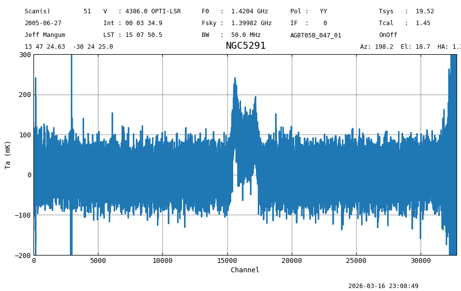
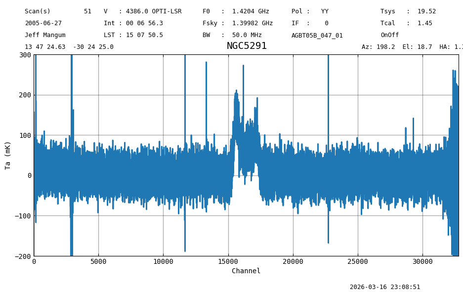
We remove the slope by baseline fitting an order 1 polynomial from the data while ignoring the channels that contain a signal. This is done using the Spectrum.baseline() method.

ta.baseline(model="poly", degree=1, include=[[3500,14000],[18000,30000]], remove=True)
ta.plot(xaxis_unit="chan", yaxis_unit="mK", ymin=-200, ymax=300, grid=True)
print(f"Stats : {fmt_str}".format(**ta[5000:14000].stats()))
print("Expect: mean: -0.0007 K median: -0.0007 K rms: 0.0358 K min: -0.13 K max: 0.15 K")

23:08:48.991 I EXCLUDING [Spectral Region, 1 sub-regions:
  (1374818364.0 Hz, 1379040470.9335938 Hz) 
, Spectral Region, 1 sub-regions:
  (1397351017.8085938 Hz, 1403454533.4335938 Hz) 
, Spectral Region, 1 sub-regions:
  (1419476261.9492188 Hz, 1424816838.1210938 Hz) 
]

Stats : mean: -0.0007 K median: -0.0007 K rms: 0.0358 K min: -0.13 K max: 0.15 K
Expect: mean: -0.0007 K median: -0.0007 K rms: 0.0358 K min: -0.13 K max: 0.15 K

Smoothing in a Few Ways

By default smoothing will also decimate the signal, to (roughly) make each channel independant from the next. This assuming the input signal had independant channels. If your input was oversampled by a factor of 2, the smoothed signal will be as well, although you can manually decimate by a different value too, for example by using decimate=8 .

Since we smooth to a gauss of FWHM 16 channels, the noise should go down by a factor of 4 (36 mK to 9 mK).

ts1 = ta.smooth('gaussian', 16)
ts1.plot(xaxis_unit="chan", yaxis_unit="mK", ymin=-200, ymax=300, grid=True)
print(f"Stats : {fmt_str}".format(**ts1[5000//16:14000//16].stats()))
print("Expect: mean: 0.0005 K median: 0.0004 K rms: 0.0075 K min: -0.02 K max: 0.03 K")

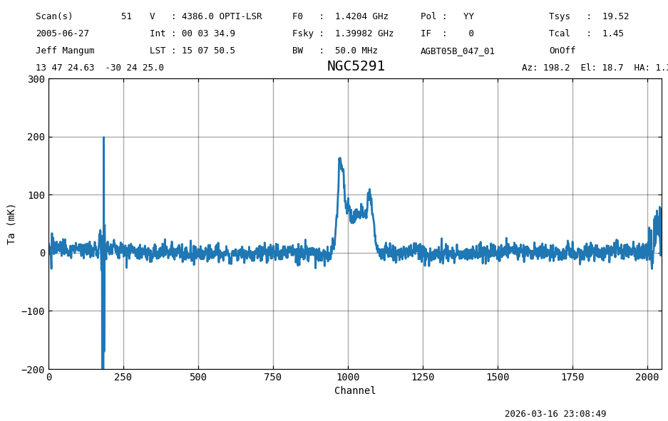
Stats : mean: -0.0007 K median: -0.0007 K rms: 0.0075 K min: -0.02 K max: 0.02 K
Expect: mean: 0.0005 K median: 0.0004 K rms: 0.0075 K min: -0.02 K max: 0.03 K

The noise is now 8 mK, very close to the improvement we expected.

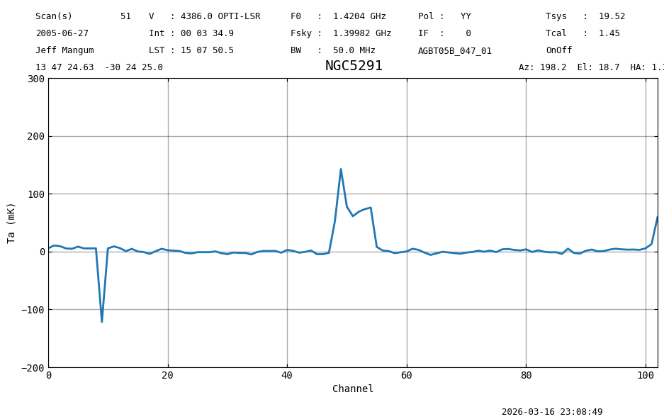
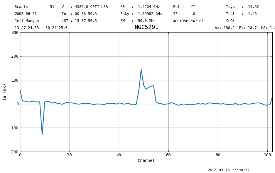
Now smoothing by 320 channels should result in a noise of \(55/\sqrt{320}\) or 2 mK. In this case we will use a box as the convolving kernel.

We will also estimate the correlation between channels by comparing the noise in the spectra with the noise in the spectra when we subtract adjacent channels (using roll=1 in Spectrum.stats).

ts2 = ta.smooth('box', 320)
ts2.plot(xaxis_unit="chan", yaxis_unit="mK", ymin=-200, ymax=300, grid=True)

print(f"Stats : {fmt_str}".format(**ts2[5000//320:14000//320].stats()))
rratio = ts2[5000//320:14000//320].stats(roll=1)["rms"]/ts2[5000//320:14000//320].stats(roll=0)["rms"]
print(f"Rolled rms/rms ratio: {rratio}")

Stats : mean: -0.0007 K median: -0.0010 K rms: 0.0023 K min: -0.01 K max: 0.00 K

Rolled rms/rms ratio: 0.7845596461442605

The noise in the smoothed spectrum is ~2 mK, as expected.

The rolled RMS ratio is very close to 1, so neighboring channels are not related. If you would decimate by 160, you would see this ratio drop. Be sure to adjust the range of channels for any new computations of the spectrum statistics (Spectrum.stats).

Smoothing the Reference (“OFF”) Scans

Under certain circumstances it can be beneficial to (boxcar) smooth the reference (OFF) signal before the usual (ON-OFF)/OFF calibration.

Technical note: if you want to achieve identical results to GBTIDL, the width of the boxcar needs to be odd.

scan_block2 = sdfits.getps(ifnum=0, plnum=0, fdnum=0, smoothref=31)
ta2 = scan_block2.timeaverage()
ta2.plot(xaxis_unit="chan", yaxis_unit="mK", ymin=100, ymax=600, grid=True)
print(f"Stats : {fmt_str}".format(**ta2[5000:10000].stats()))   # avoid spikes
print("Expect: mean: 0.2667 K median: 0.2666 K rms: 0.02536 K min: 0.18 K max: 0.35 K")

Stats : mean: 0.2667 K median: 0.2666 K rms: 0.0254 K min: 0.18 K max: 0.35 K
Expect: mean: 0.2667 K median: 0.2666 K rms: 0.02536 K min: 0.18 K max: 0.35 K

When smoothing the reference spectra, the noise in the time average of the calibrated spectrum is 25 mK. For a given value of the smoothref=\(N\) the improvement is

\[ \sqrt{\frac{N+1}{2N}} \]

Given that the RMS was 36 mK we would expect \(\sqrt(32/62) \approx 0.72\) times, or 26 mK. At best this will give about 30% improvement. See our sdmath for more details.

We repeat the baseline subtraction using the same model.

ta2.baseline(model="poly", degree=1, exclude=[(14000,18000)], remove=True)
ta2.plot(xaxis_unit="chan", yaxis_unit="mK", ymin=-200, ymax=300, grid=True)
print(f"Stats : {fmt_str}".format(**ta2[5000:14000].stats()))
print("Expect: mean: 0.0009 K median: 0.0007 K rms: 0.0270 K min: -0.19 K max: 0.50 K")

23:08:51.565 I EXCLUDING [Spectral Region, 1 sub-regions:
  (1397351017.8085938 Hz, 1403454533.4335938 Hz) 
]

Stats : mean: 0.0009 K median: 0.0007 K rms: 0.0270 K min: -0.19 K max: 0.50 K
Expect: mean: 0.0009 K median: 0.0007 K rms: 0.0270 K min: -0.19 K max: 0.50 K

We could smooth this spectrum the normal way, as was done a few cells ago, and not much difference is visible, except for the noise.

ts3 = ta2.smooth('box', 320)
ts3.plot(xaxis_unit="chan", yaxis_unit="mK", ymin=-200, ymax=300, grid=True)
print(f"Stats : {fmt_str}".format(**ts3[5000//320:14000//320].stats()))
rratio = ts3[5000//320:14000//320].stats(roll=1)["rms"]/ts3[5000//320:14000//320].stats(roll=0)["rms"]
print(f"Rolled rms/rms ratio: {rratio}")

Stats : mean: 0.0009 K median: 0.0007 K rms: 0.0023 K min: -0.00 K max: 0.01 K

Rolled rms/rms ratio: 0.7802633164999715

The RMS has gone down (2.4 mK to 2.3 mK), but the signal correlation has also increased from 1.06 to 1.10. This increase is due to the added correlation of the reference smoothing.

Successive Smoothing

Smoothing with a Gaussian twice in a row should be the same as smoothing with a single Gaussian of the square root of the sum of their squares. Note that the width is the final width (FWHM) of the smoothing operation. We need to ignore decimation here, which is the third argument (decimate=-1), otherwise the spectra will have a different number of channels.

We plot the difference between the two smoothing routes, which is perhaps surprisingly still below 1e-8. It is not closer to 0 due to the finite range the Gaussian is sampled (to 4 sigma).

ts5a = ta.smooth('gaussian', width=3, decimate=-1).smooth('gaussian', width=5, decimate=-1)
ts5b = ta.smooth('gaussian', width=5, decimate=-1)
diff = ts5a-ts5b
diff.plot(ymin=-0.00001, ymax=0.00001)

fmt_str = "mean: {mean:.4g} median: {median:.4g} rms: {rms:.4g} min: {min:.2g} max: {max:.2g}"
print(f"Stats : {fmt_str}".format(**diff[5000:14000].stats()))

Stats : mean: -2.945e-10 K median: 4.285e-09 K rms: 7.291e-07 K min: -2.8e-06 K max: 2.7e-06 K

Final Stats

Finally, at the end we compute some statistics over a spectrum, merely as a checksum if the notebook is reproducible.

ts5b.check_stats(0.04618235 * u.K)

23:08:53.308 I rms is OK