Modifying Metadata#
This notebook shows how to modify the metadata of an SDFITS file using dysh.
Background#
We will use a practical example. For observations with the GBT it is recommended to observe a flux density calibrator (see e.g., Perley & Butler 2017 for a list of calibrator sources and their flux densities) with the same configuration as that used for the science observations. The reason being that the values of the temperature equivalent power of the noise diodes stored in the SDFITS files can be out of date.
In this example we won’t use observations of a flux density calibrator, but instead we will use the analysis of Goddy et al (2020). They find that the temperature stored in the SDFITS files is on average lower than the measured values, so that the temperature must be corrected by 20%
Dysh commands#
The following dysh commands are introduced (leaving out all the function arguments):
  filename = dysh_data()
  sdf = GBTFITSLoad()
  sdf.select()
  sb = sdf.getps()
  ta = sb.timeaverage()
  ta.baseline()
  ta.average()
  ta.plot()
  ta_plt.savefig()
Loading Modules#
We start by loading the modules we will use for this example.
# These modules are required for working with the data.
from dysh.fits.gbtfitsload import GBTFITSLoad
from dysh.log import init_logging
from astropy import units as u

# These modules are used for file I/O
from dysh.util.files import dysh_data
from pathlib import Path
Setup#
We start the dysh logging, so we get more information about what is happening.
This is only needed if working on a notebook.
If using the CLI through the dysh command, then logging is setup for you.
init_logging(2)

# also create a local "output" directory where temporary notebook files can be stored.
output_dir = Path.cwd() / "output"
output_dir.mkdir(exist_ok=True)
Data retrieval#
We download the data we will use for this example, if necessary.
filename = dysh_data(test="getps")
23:07:03.908 I Resolving test=getps -> AGBT05B_047_01/AGBT05B_047_01.raw.acs/
Data loading#
We load the data and inspect its contents.
sdfits = GBTFITSLoad(filename)
23:07:03.958 I Index loaded from .index file (44/93 columns). Missing columns (TCAL, WCS, calibration metadata, etc.) will be automatically loaded from FITS file when first accessed.
sdfits.summary()
| SCAN | OBJECT | VELOCITY | PROC | PROCSEQN | RESTFREQ | # IF | # POL | # INT | # FEED | AZIMUTH | ELEVATION |
|---|---|---|---|---|---|---|---|---|---|---|---|
| 51 | NGC5291 | 4386.0 | OnOff | 1 | 1.420405 | 1 | 2 | 11 | 1 | 198.3431 | 18.6427 |
| 52 | NGC5291 | 4386.0 | OnOff | 2 | 1.420405 | 1 | 2 | 11 | 1 | 198.9306 | 18.7872 |
| 53 | NGC5291 | 4386.0 | OnOff | 1 | 1.420405 | 1 | 2 | 11 | 1 | 199.3305 | 18.3561 |
| 54 | NGC5291 | 4386.0 | OnOff | 2 | 1.420405 | 1 | 2 | 11 | 1 | 199.9157 | 18.4927 |
| 55 | NGC5291 | 4386.0 | OnOff | 1 | 1.420405 | 1 | 2 | 11 | 1 | 200.3042 | 18.0575 |
| 56 | NGC5291 | 4386.0 | OnOff | 2 | 1.420405 | 1 | 2 | 11 | 1 | 200.8906 | 18.1860 |
| 57 | NGC5291 | 4386.0 | OnOff | 1 | 1.420405 | 1 | 2 | 11 | 1 | 202.3275 | 17.3853 |
| 58 | NGC5291 | 4386.0 | OnOff | 2 | 1.420405 | 1 | 2 | 11 | 1 | 202.9192 | 17.4949 |
Metadata inspection#
Now we inspect the current noise diode temperature stored in the SDFITS file, and some additional related parameters.
sdfits["TCAL", "PLNUM", "CAL", "INTNUM"]
23:07:03.981 I Column(s) ['TCAL'] not available in .index file. Loading from FITS file(s)...
| TCAL | PLNUM | CAL | INTNUM | |
|---|---|---|---|---|
| 0 | 1.424292 | 1 | T | 0 |
| 1 | 1.424292 | 1 | F | 0 |
| 2 | 1.452650 | 0 | T | 0 |
| 3 | 1.452650 | 0 | F | 0 |
| 4 | 1.424292 | 1 | T | 1 |
| ... | ... | ... | ... | ... |
| 347 | 1.452650 | 0 | F | 9 |
| 348 | 1.424292 | 1 | T | 10 |
| 349 | 1.424292 | 1 | F | 10 |
| 350 | 1.452650 | 0 | T | 10 |
| 351 | 1.452650 | 0 | F | 10 |
352 rows × 4 columns
For polarization 0 the noise diode temperature is 1.452650 K and for polarization 1 it is 1.424292 K.
We will calibrate the data using these values to compare after we update the noise diode temperature. We use position switching calibration, then we time average all the scans and remove an order 1 polynomial.
ps_original = sdfits.getps(plnum=0, ifnum=0, fdnum=0).timeaverage()
ps_original.baseline(degree=1, remove=True)
23:07:05.564 I EXCLUDING None
Metadata update#
Now we update the temperature of the noise diode by multiplying by 1.2.
sdfits["TCAL"] *= 1.2
/home/docs/checkouts/readthedocs.org/user_builds/dysh/checkouts/release-1.0.0/src/dysh/fits/gbtfitsload.py:4184: UserWarning: Changing an existing SDFITS column TCAL
  warnings.warn(f"Changing an existing SDFITS column {items}")  # noqa: B028
/home/docs/checkouts/readthedocs.org/user_builds/dysh/checkouts/release-1.0.0/src/dysh/fits/sdfitsload.py:1496: UserWarning: Changing an existing SDFITS column TCAL
  warnings.warn(f"Changing an existing SDFITS column {items}")  # noqa: B028
Now we check that the values were updated.
sdfits["TCAL", "PLNUM"]
| TCAL | PLNUM | |
|---|---|---|
| 0 | 1.70915 | 1 |
| 1 | 1.70915 | 1 |
| 2 | 1.74318 | 0 |
| 3 | 1.74318 | 0 |
| 4 | 1.70915 | 1 |
| ... | ... | ... |
| 347 | 1.74318 | 0 |
| 348 | 1.70915 | 1 |
| 349 | 1.70915 | 1 |
| 350 | 1.74318 | 0 |
| 351 | 1.74318 | 0 |
352 rows × 2 columns
The values were updated. We proceed with the data reduction.
ps_updated = sdfits.getps(plnum=0, ifnum=0, fdnum=0).timeaverage()
ps_updated.baseline(degree=1, remove=True)
23:07:06.359 I EXCLUDING None
Now plot and compare the result. Since the antenna temperature is directly proportional to the temperature of the noise diode, now the line profile after the update should be 20% brighter than without the update.
ps_original.plot(ymin=-0.5, ymax=0.3)
ps_updated.plot(ymin=-0.5, ymax=0.3)
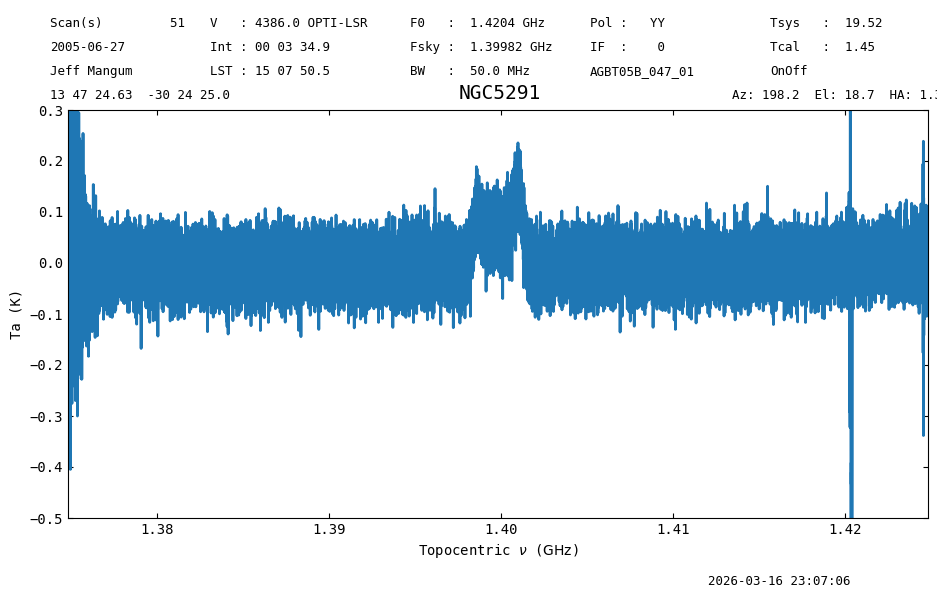
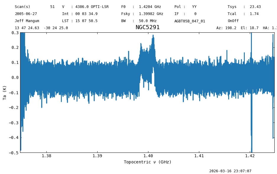
<dysh.plot.specplot.SpectrumPlot at 0x7f511532ae30>
Final Stats#
Finally, at the end we compute some statistics over a spectrum, merely as a checksum if the notebook is reproducible.
ps_updated.check_stats(0.07192832 * u.K)
23:07:07.310 I rms is OK