Modifying the Default Values for Surface Error and Aperture Efficiency#
This notebook shows how you can modify the defaults for surface error and aperture efficiency. We encourage users of the GBT to rely on the Observatory-measured values and functions for surface error and aperture efficiency, which are implemented in dysh. However, advanced users may wish to modify the values or functions; this example shows how to do that.
Refresher on Aperture Efficiency and Brightness Scales#
The aperture efficiency \(\eta_a\) is determined by:
where \(\eta_0\) is the long wavelength aperture efficiency, \(G(ZD)\) is the gain correction factor at a zenith distance \(ZD\), \(\epsilon\) is the surface error, and \(\lambda\) is the wavelength.
To scale antenna temperature \(T_a\) to brightness tempeature \(T_a^*\):
where \(\tau\) is the zenith opacity, \(A\) is the airmass, and \(\eta_l\) is the loss efficiency. To scale to flux \(S_\nu\)
where \(k\) is Boltzmann’s constant is \(A_p\) is the physical aperture of the telescope.
What dysh Does#
When you calibrate and scale data through, e.g.
GBTFITSLoad.getps,
dysh uses the GBTGainCorrection class to manage the calculations described above. GBTGainCorrection maintains \(G(ZD)\) and surface error as a function of date as derived in
GBT Memo 301.
You can provide your own values for \(\eta_a\) or \(\epsilon\) in the standard calibration routines (you must provide \(\tau\)).
Dysh commands#
The following dysh commands are introduced (leaving out all the function arguments):
  filename = dysh_data()
  sdf = GBTFITSLoad()
  sb = sdf.getps()
  ta = sb.timeaverage()
Loading Modules#
We start by loading the modules we will use for the data reduction.
# These modules are required for the data reduction.
from dysh.fits.gbtfitsload import GBTFITSLoad
from astropy import units as u
import numpy as np
from dysh.log import init_logging

# These modules are used for file I/O
from dysh.util.files import dysh_data
from pathlib import Path
Setup#
dysh uses a logger to communicate. If you are working in the command line, then the logging is setup for you. If you are working in a jupyter lab instance, then you need to set it up. You can do so using the init_logging function imported above. As an argument, init_logging takes a number, the verbosity level. level 0 is for error messages only, 1 for warning, 2 for info and 3 for debug. Here we set it to level 2.
init_logging(2)

# also create a local "output" directory where temporary notebook files can be stored.
output_dir = Path.cwd() / "output"
output_dir.mkdir(exist_ok=True)
Data Retrieval#
Download the example SDFITS data, if necessary.
filename = dysh_data(test="getps")
23:03:42.329 I Resolving test=getps -> AGBT05B_047_01/AGBT05B_047_01.raw.acs/
Data Loading#
Next, we use GBTFITSLoad to load the data, and then its summary method to inspect its contents.
sdfits = GBTFITSLoad(filename)
23:03:42.381 I Index loaded from .index file (44/93 columns). Missing columns (TCAL, WCS, calibration metadata, etc.) will be automatically loaded from FITS file when first accessed.
sdfits.summary()
| SCAN | OBJECT | VELOCITY | PROC | PROCSEQN | RESTFREQ | # IF | # POL | # INT | # FEED | AZIMUTH | ELEVATION |
|---|---|---|---|---|---|---|---|---|---|---|---|
| 51 | NGC5291 | 4386.0 | OnOff | 1 | 1.420405 | 1 | 2 | 11 | 1 | 198.3431 | 18.6427 |
| 52 | NGC5291 | 4386.0 | OnOff | 2 | 1.420405 | 1 | 2 | 11 | 1 | 198.9306 | 18.7872 |
| 53 | NGC5291 | 4386.0 | OnOff | 1 | 1.420405 | 1 | 2 | 11 | 1 | 199.3305 | 18.3561 |
| 54 | NGC5291 | 4386.0 | OnOff | 2 | 1.420405 | 1 | 2 | 11 | 1 | 199.9157 | 18.4927 |
| 55 | NGC5291 | 4386.0 | OnOff | 1 | 1.420405 | 1 | 2 | 11 | 1 | 200.3042 | 18.0575 |
| 56 | NGC5291 | 4386.0 | OnOff | 2 | 1.420405 | 1 | 2 | 11 | 1 | 200.8906 | 18.1860 |
| 57 | NGC5291 | 4386.0 | OnOff | 1 | 1.420405 | 1 | 2 | 11 | 1 | 202.3275 | 17.3853 |
| 58 | NGC5291 | 4386.0 | OnOff | 2 | 1.420405 | 1 | 2 | 11 | 1 | 202.9192 | 17.4949 |
Data Reduction#
We calibrate a few scans of the position switched observations, giving a value for zenith_opacity but leaving dysh to calculate the aperture efficiency.
We will calibrate scans 51, 53 and 55.
We use a zenith opacity of 0.08, but the exact value is not important here.
And, we request that the data be calibrated to units of flux, so that the aperture efficiency goes into the calculations.
scans = [51,53,55]
ps_scan_block = sdfits.getps(scan=scans, ifnum=0, plnum=0, fdnum=0, units="flux",
                             zenith_opacity=0.08)
Providing Aperture Efficiency or Surface Error#
Now, we calibrate the same data, but we provide a value for the aperture efficiency.
We use a value of \(25\%\) (ap_eff=0.25).
ps_scan_block_ap_eff = sdfits.getps(scan=scans, ifnum=0, plnum=0, fdnum=0, units="flux",
                                    zenith_opacity=0.08, ap_eff=0.25)
Alternatively, one could specify the surface error using the surface_error argument.
The value of the surface_error must be a quantity with units compatible with a length.
(You can’t give both surface error and aperture efficiency because the latter is computed from the former.)
ps_scan_block_surf_err = sdfits.getps(scan=scans, ifnum=0, plnum=0, fdnum=0, units="flux",
                                      zenith_opacity=0.08, surface_error=400*u.micron)
Now we print the different \(\eta_a\) for the first scan in each ScanBlock.
You can see that at this wavelength, the surface error does not have much of an effect because \(\epsilon << \lambda\). (400 \(\mu\)m vs. 21 cm)
print(f"{np.mean(ps_scan_block[0].ap_eff):.4f},{np.mean(ps_scan_block_ap_eff[0].ap_eff):.4f},{np.mean(ps_scan_block_surf_err[0].ap_eff):.4f}")
0.6095,0.2500,0.6095
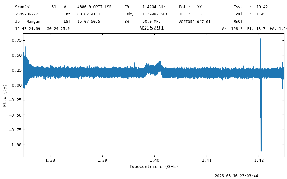
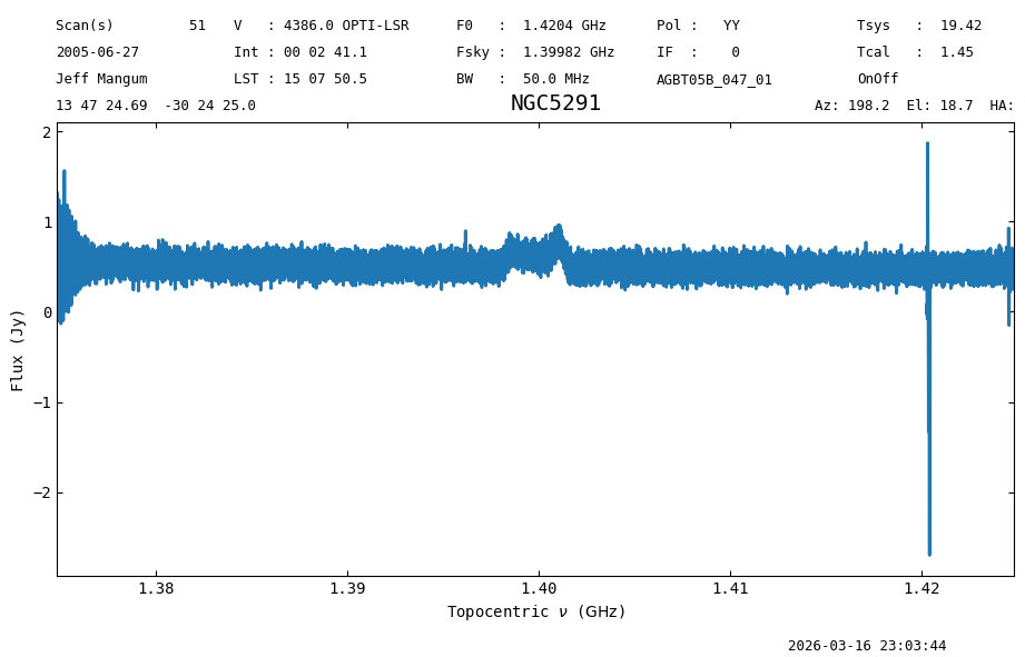
But the aperture efficiency does make a difference in the derived flux.
a = ps_scan_block.timeaverage()
print(f"S_nu = {a.stats()['median']:.3}")
a.plot();
S_nu = 0.209 Jy
b = ps_scan_block_ap_eff.timeaverage()
print(f"S_nu = {b.stats()['median']:.3}")
b.plot();
S_nu = 0.508 Jy
The weighted average aperture efficiency, surface error, and zenith opacity are stored in the Spectrum metadata.
print(f"eta = {a.meta['AP_EFF']:.3f}, epsilon = {a.meta['SURF_ERR']:.1f} {a.meta['SE_UNIT']}, tau = {a.meta['TAU_Z']:.2f}")
eta = 0.608, epsilon = 440.0 micron, tau = 0.08
What if I want to change \(G(ZD)\) or the surface error model?#
This is advanced usage and requires you to fork or clone dysh, then modify src/dysh/data/gaincorrection.tab. If you have questions, consult with a dysh developer.
Final Stats#
Finally, at the end we compute some statistics over a spectrum, merely as a checksum if the notebook is reproducible.
b.check_stats(0.11950689 * u.Jy)
23:03:45.304 I rms is OK