Working With Repeated Scan Numbers#
This notebook shows how to work with repeated scan numbers. It uses data from an RFI scan, a trimmed down version.
In this case there are two occurrences of scan 2. The two used a different number of channels, so they end up in different binary tables. We will use summary to determine how to uniquely identify them, and then gettp to retrieve the data.
Dysh Commands#
The following dysh commands are (re)introduced (leaving out all the function arguments):
filename = dysh_data()
sdf = GBTFITSLoad()
sdf.summary()
sb = sdf.getps()
ta = sb.timeaverage()
ta.plot()
Loading Modules#
We start by loading the modules we will use for the recipe.
# These modules are required for the data reduction.
from dysh.fits.gbtfitsload import GBTFITSLoad
from dysh.log import init_logging

# These modules are used for file I/O
from dysh.util.files import dysh_data
from pathlib import Path
Setup#
We start the dysh logging, so we get more information about what is happening. This is only needed if working on a notebook. If using the CLI through the dysh command, then logging is setup for you.
init_logging(2)

# also create a local "output" directory where temporary notebook files can be stored.
output_dir = Path.cwd() / "output"
output_dir.mkdir(exist_ok=True)
Data Retrieval#
Download the example SDFITS data’
filename = dysh_data(example="repeated")
23:08:33.122 I Resolving example=repeated -> repeated-scans/data/TRFI_090125_S1.raw.vegas/TRFI_090125_S1.raw.vegas.testtrim.fits
23:08:33.122 I url: http://www.gb.nrao.edu/dysh//example_data/repeated-scans/data/TRFI_090125_S1.raw.vegas/TRFI_090125_S1.raw.vegas.testtrim.fits
Downloading TRFI_090125_S1.raw.vegas.testtrim.fits from http://www.gb.nrao.edu/dysh//example_data/repeated-scans/data/TRFI_090125_S1.raw.vegas/TRFI_090125_S1.raw.vegas.testtrim.fits
23:08:33.451 I Starting download...
23:08:34.115 I Saved TRFI_090125_S1.raw.vegas.testtrim.fits to TRFI_090125_S1.raw.vegas.testtrim.fits
Retrieved TRFI_090125_S1.raw.vegas.testtrim.fits
Data Loading#
Next, we use GBTFITSLoad to load the data, and then its summary method to inspect its contents.
sdfits = GBTFITSLoad(filename)
sdfits.summary()
| SCAN | OBJECT | VELOCITY | PROC | PROCSEQN | RESTFREQ | # IF | # POL | # INT | # FEED | AZIMUTH | ELEVATION |
|---|---|---|---|---|---|---|---|---|---|---|---|
| 2 | rfiscan1 | 0.0 | Track | 1 | 2.15 | 1 | 1 | 4 | 1 | 15.3022 | 44.5177 |
| 2 | rfiscan2 | 0.0 | Track | 1 | 0.75 | 1 | 1 | 4 | 1 | 172.2867 | 44.5177 |
The summary tells us there are two instances of scan 2. How can we tell them apart?
Identifying Data#
By default summary will separate the information by scan number (SCAN), project ID (PROJID) and binary table (BINTABLE).
Since we see there are two occurrences of scan 2, it means one of those columns has different values for each of them.
We can show more columns by using the add_columns argument of summary to inspect their values.
sdfits.summary(add_columns="BINTABLE, PROJID")
| SCAN | OBJECT | VELOCITY | PROC | PROCSEQN | RESTFREQ | # IF | # POL | # INT | # FEED | AZIMUTH | ELEVATION | BINTABLE | PROJID |
|---|---|---|---|---|---|---|---|---|---|---|---|---|---|
| 2 | rfiscan1 | 0.0 | Track | 1 | 2.15 | 1 | 1 | 4 | 1 | 15.3022 | 44.5177 | 0 | TRFI_090125_S1 |
| 2 | rfiscan2 | 0.0 | Track | 1 | 0.75 | 1 | 1 | 4 | 1 | 172.2867 | 44.5177 | 1 | TRFI_090125_S1 |
This shows that the data have the same project ID, and different binary tables. We can use the BINTABLE column to uniquely identify the data. The first occurrence has BINATBLE 0 and the second 1. It is important to note that the BINTABLE column gets a value depending on the contents of the file at the time of loading, so its value is not absolute. If you were working with the full data set the BINTABLE values would be different.
Retrieving Data#
Now that we know how to identify the scans we can use this information to retrieve the data we want. We pass the bintable keyword to gettp to get the data we want.
For the first occurrence of scan 2 we use
tpsb1 = sdfits.gettp(scan=2, ifnum=0, plnum=0, fdnum=0, bintable=0)
For the second occurrence we use
tpsb2 = sdfits.gettp(scan=2, ifnum=0, plnum=0, fdnum=0, bintable=1)
Now we plot the two together to show that they are indeed different.
tpsb1_plt = tpsb1.timeaverage().plot(oshow=tpsb2.timeaverage(), xaxis_unit="GHz")
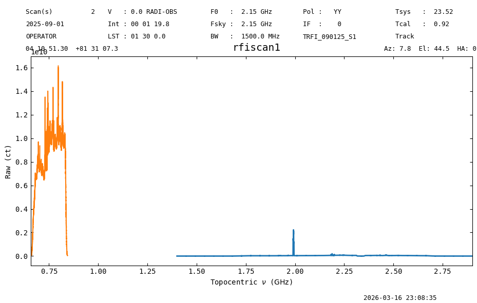
We can clearly see that they have different rest frequencies, though only one can be plotted in the header (as F0)
Final Stats#
Finally, at the end we compute some statistics over a spectrum, merely as a checksum if the notebook is reproducible.
tpsb1.timeaverage().check_stats(81581261.43976656)
23:08:36.162 I rms is OK (no unit was given, assumed ct)
tpsb2.timeaverage().check_stats(3.06388519e+09)
23:08:36.295 I rms is OK (no unit was given, assumed ct)