Vane Calibration#
This example shows how to calibrate data that uses a vane (or a hot load) to determine the system temperature. In the case of the GBT this applies mainly to Argus, although the Q-band receiver also has a vane. For the background on the calibration please refer to Frayer et al. 2019.
You can find a copy of this tutorial as a Jupyter notebook here or download it by right clicking here and selecting “Save Link As”.
Loading Modules#
We start by loading the modules we will use for this example.
For display purposes, we use the static (non-interactive) matplotlib backend in this tutorial.
However, you can tell matplotlib to use the ipympl backend to enable interactive plots.
This is only needed if working on jupyter lab or notebook.
# These modules are required for the data reduction.
from dysh.fits import GBTFITSLoad

# These are only needed if working on a notebook.
#%matplotlib ipympl # Uncomment for interactive figures.
from dysh.log import init_logging

# These modules are only used to download the data.
from pathlib import Path
from dysh.util.download import from_url
Setup#
We start the dysh logging, so we get more information about what is happening.
This is only needed if working on a notebook.
If using the CLI through the dysh command, then logging is setup for you.
init_logging(2)
Data Retrieval#
Download the example SDFITS data, if necessary.
url = "http://www.gb.nrao.edu/dysh/example_data/fs-Argus/data/AGBT20B_295_02.raw.vegas/AGBT20B_295_02.raw.vegas.A.fits"
savepath = Path.cwd() / "data"
savepath.mkdir(exist_ok=True) # Create the data directory if it does not exist.
filename = from_url(url, savepath)
21:07:43.975 I Starting download...
21:07:45.419 I Saved AGBT20B_295_02.raw.vegas.A.fits to /home/docs/checkouts/readthedocs.org/user_builds/dysh/checkouts/release-0.11.5/docs/source/tutorials/examples/data/AGBT20B_295_02.raw.vegas.A.fits
Data Loading#
Next, we use GBTFITSLoad to load the data, and then its summary method to inspect its contents.
sdfits = GBTFITSLoad(filename)
sdfits.summary()
| SCAN | OBJECT | VELOCITY | PROC | PROCSEQN | RESTFREQ | DOPFREQ | # IF | # POL | # INT | # FEED | AZIMUTH | ELEVATION |
|---|---|---|---|---|---|---|---|---|---|---|---|---|
| 10 | VANE | 65.0 | Track | 1 | 93.173777 | 93.173777 | 1 | 1 | 25 | 2 | 166.9878 | 43.5400 |
| 11 | SKY | 65.0 | Track | 1 | 93.173777 | 93.173777 | 1 | 1 | 25 | 2 | 166.9875 | 43.5399 |
| 12 | G24.789 | 65.0 | Track | 1 | 93.173777 | 93.173777 | 1 | 1 | 151 | 2 | 167.4363 | 43.6122 |
This is a frequency switched observation with Argus. The first two scans, 10 and 11, are observations of the vane and the “cold” sky. The next scan, 12, are the observations of the target using frequency switching.
Data Reduction#
To calibrate data using a vane we can use the same methods as with any other observations, with the difference that we must specify the vane argument.
This argument can be an integer, with the scan number of the vane observations (in this case scan 10), or it can be a VaneSpectrum object.
Calibration with Vane#
We will show how to calibrate the data providing a scan number for the vane argument.
We call getfs with vane=10.
If working from one of the GBO data reduction hosts, this will initialize a VaneSpectrum and determine the zenith opacity and atmospheric temperature from the CLEO weather forecast scripts.
If working from elsewhere, then by default these values are not known and the vane calibration will use an approximation to determine the system temperature (equation (23) in Frayer et al. 2019).
For this data set we know that feeds 10 and 8 are available, we use fdnum=10, and only a single spectral window and polarization are available, so we use ifnum=0 and plnum=0.
ta = sdfits.getfs(scan=12, ifnum=0, plnum=0, fdnum=10, vane=10).timeaverage()
21:07:45.682 I Vane calibrated data will be calibrated to Ta* units by default.
21:07:46.892 I Weather forecast not available.
21:07:47.036 I Ignoring 1 blanked integration(s).
21:07:47.166 I Vane temperature (twarm): 400.15 K
21:07:47.167 I No zenith opacity nor atmospheric temperature available. Will approximate the calibration temperature to the vane temperature 400.15 K
21:07:47.168 I Mean calibration temperature (tcal): 400.15 K
The above messages tells us what values for the different parameters required to determine the system temperature were adopted.
Next, we plot the calibrated spectrum.
plot = ta.plot()
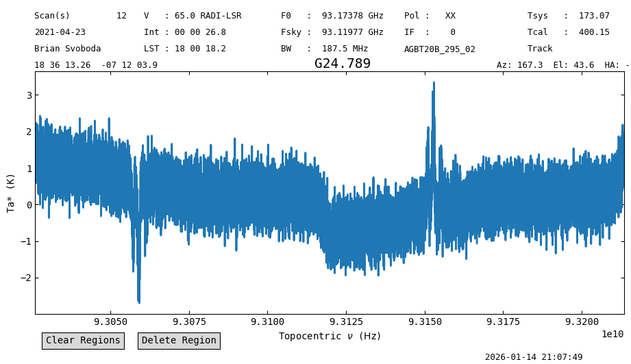
We see a clear signal at about 93.150 GHz, and it’s “ghost” at 93.055 GHz.
Changing default values#
The parameters required to determine the system temperature using a vane are: the zenith opacity (zenith_opacity), vane temperature (t_warm), atmospheric temperature (t_atm) and background temperature (t_bkg).
From these a calibration temperature (t_cal) is derived.
These can be modified by providing values for them as arguments to the calibration method.
In the following code, we modify the first four parameters used to derive the calibration temperature.
We set zenith_opacity=0.01 in nepers, t_warm=583 in K, t_atm=260 in K and t_bkg=3.
We use a higher vane temperature so we can see the difference when comparing the results.
ta2 = sdfits.getfs(scan=12, ifnum=0, plnum=0, fdnum=10, vane=10,
                   zenith_opacity=0.01,
                   t_warm=583,
                   t_atm=260,
                   t_bkg=3,
                  ).timeaverage()
21:07:49.607 I Vane calibrated data will be calibrated to Ta* units by default.
21:07:50.253 I Weather forecast not available.
21:07:50.382 I Ignoring 1 blanked integration(s).
21:07:50.507 I Vane temperature (twarm): 583.00 K
21:07:50.508 I Mean calibration temperature (tcal): 584.97 K
Now we plot both results on top of each other, with the increased vane temperature spectrum in blue and the original spectrum in orange.
plot2 = ta2.plot()
plot2.oshow(ta)
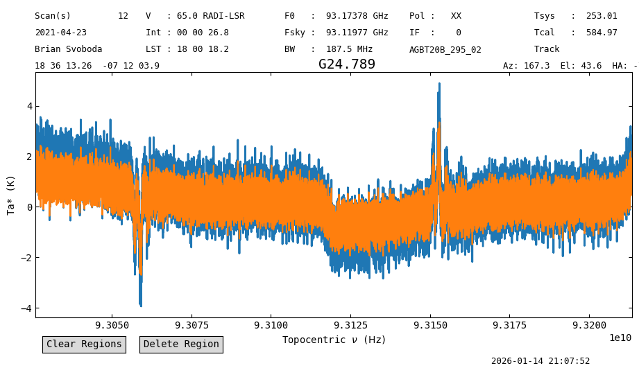
The effect of having a larger vane temperature is to increase the derived system temperature, so the resulting spectrum is scaled up.
We can check the system temperature by inspecting the “TSYS” item of the Spectrum.meta dictionary.
print(ta.meta["TSYS"], ta2.meta["TSYS"])
173.0724666317342 253.01146158520933
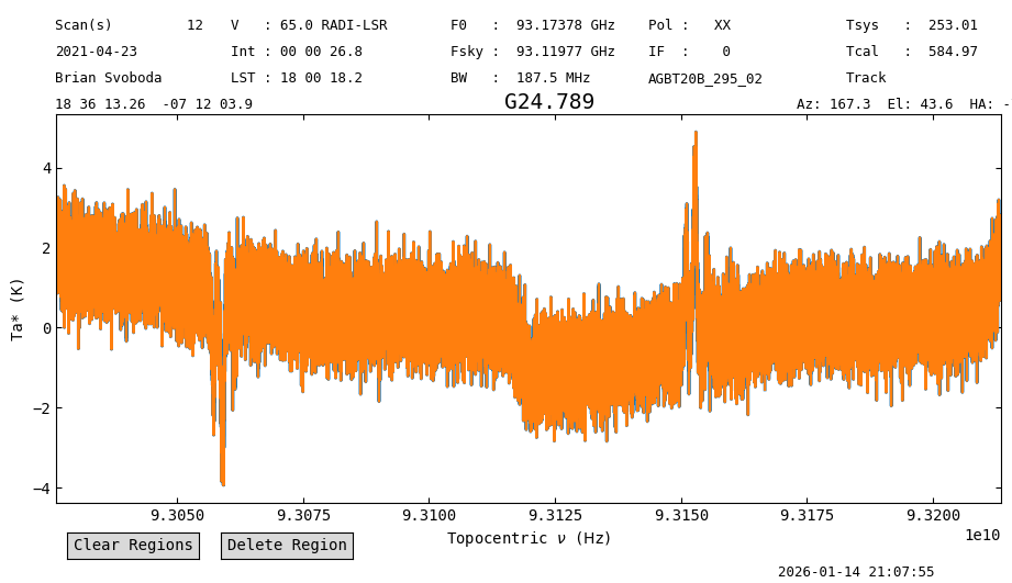
Alternatively, we can directly provide a value for the calibration temperature, and get the same result. From the output of the previous example, we had a calibration temperature of 584.97 K.
ta3 = sdfits.getfs(scan=12, ifnum=0, plnum=0, fdnum=10, vane=10,
                   t_cal=584.97
                  ).timeaverage()
21:07:52.817 I Vane calibrated data will be calibrated to Ta* units by default.
21:07:53.326 I Weather forecast not available.
21:07:53.453 I Ignoring 1 blanked integration(s).
We plot this and the previous result on top of each other to confirm that they are the same.
plot3 = ta3.plot()
plot3.oshow(ta2)
Creating a VaneSpectrum Object#
For more control, or developing alternative data reduction approaches, one could create a VaneSpectrum object directly.
There are two ways of doing so, using getvane, or directly instanciating a VaneSpectrum object by directly providing the input values, or from a Spectrum object using VaneSpectrum.from_spectrum.
Here we will show how to use getvane.
The arguments are the same as those provided for the calibration.
vane = sdfits.getvane(scan=10, ifnum=0, plnum=0, fdnum=10,
                      zenith_opacity=0.01,
                      t_warm=583,
                      t_atm=260,
                      t_bkg=3)
21:07:56.390 I Weather forecast not available.
The calibration temperature can be obtained using the VaneSpectrum.get_tcal method.
This takes as input a reference Spectrum.
For example:
ref = sdfits.gettp(scan=11, ifnum=0, plnum=0, fdnum=10).timeaverage()
21:07:56.459 I Using TSYS column
vane.get_tcal(ref)
21:07:56.769 I Vane temperature (twarm): 583.00 K
21:07:56.771 I Mean calibration temperature (tcal): 584.98 K
np.float64(584.9782633701202)
And the system temperature using the VaneSpectrum.get_tsys method, which also takes as input a reference Spectrum.
vane.get_tsys(ref)
21:07:56.779 I Vane temperature (twarm): 583.00 K
21:07:56.780 I Mean calibration temperature (tcal): 584.98 K
np.float64(250.1676896502541)
As mentioned earlier, it is also possible to directly provide a VaneSpectrum to the calibration methods. In this case, the additional parameters (t_warm, t_atm, t_bkg and t_cal are ignored).
For example:
ta4 = sdfits.getfs(scan=12, ifnum=0, plnum=0, fdnum=10, vane=vane).timeaverage()
plot4 = ta4.plot()
21:07:56.788 I Vane calibrated data will be calibrated to Ta* units by default.
21:07:56.790 I Will use a zenith opacity of 0.01 nepers. Taken from vane.
21:07:56.921 I Ignoring 1 blanked integration(s).
21:07:57.050 I Vane temperature (twarm): 583.00 K
21:07:57.052 I Mean calibration temperature (tcal): 584.97 K

We also note that when providing the vane argument during calibration, the system temperature argument t_sys is ignored.