Saving Data to External Files#
This notebook gives examples of how to write out selected data from GBTFitsLoad and how to save
Spectrum,
Scan, and
ScanBlock to different formats.
You can find a copy of this tutorial as a Jupyter notebook here or download it by right clicking here and selecting “Save Link As”.
Loading Modules#
We start by loading the modules we will use for this example.
For display purposes, we use the static (non-interactive) matplotlib backend in this tutorial. However, you can tell matplotlib to use the ipympl backend to enable interactive plots. This is only needed if working on jupyter lab or notebook.
# Set interactive plots in jupyter.
#%matplotlib ipympl

# These modules are required for loading and reading data.
from dysh.fits.gbtfitsload import GBTFITSLoad
from dysh.spectra.spectrum import Spectrum

# We will use matplotlib for plotting.
import matplotlib.pyplot as plt

# These modules are only used to download the data.
from pathlib import Path
from dysh.util.download import from_url
Data Retrieval#
Download the example SDFITS data, if necessary.
url = "http://www.gb.nrao.edu/dysh/example_data/positionswitch/data/AGBT05B_047_01/AGBT05B_047_01.raw.acs/AGBT05B_047_01.raw.acs.fits"
savepath = Path.cwd() / "data"
savepath.mkdir(exist_ok=True) # Create the data directory if it does not exist.
filename = from_url(url, savepath)
Data Loading#
Next, we use GBTFITSLoad to load the data, and then its summary method to inspect its contents.
sdfits = GBTFITSLoad(filename)
sdfits.summary()
| SCAN | OBJECT | VELOCITY | PROC | PROCSEQN | RESTFREQ | DOPFREQ | # IF | # POL | # INT | # FEED | AZIMUTH | ELEVATION |
|---|---|---|---|---|---|---|---|---|---|---|---|---|
| 51 | NGC5291 | 4386.0 | OnOff | 1 | 1.420405 | 1.420405 | 1 | 2 | 11 | 1 | 198.3431 | 18.6427 |
| 52 | NGC5291 | 4386.0 | OnOff | 2 | 1.420405 | 1.420405 | 1 | 2 | 11 | 1 | 198.9306 | 18.7872 |
| 53 | NGC5291 | 4386.0 | OnOff | 1 | 1.420405 | 1.420405 | 1 | 2 | 11 | 1 | 199.3305 | 18.3561 |
| 54 | NGC5291 | 4386.0 | OnOff | 2 | 1.420405 | 1.420405 | 1 | 2 | 11 | 1 | 199.9157 | 18.4927 |
| 55 | NGC5291 | 4386.0 | OnOff | 1 | 1.420405 | 1.420405 | 1 | 2 | 11 | 1 | 200.3042 | 18.0575 |
| 56 | NGC5291 | 4386.0 | OnOff | 2 | 1.420405 | 1.420405 | 1 | 2 | 11 | 1 | 200.8906 | 18.1860 |
| 57 | NGC5291 | 4386.0 | OnOff | 1 | 1.420405 | 1.420405 | 1 | 2 | 11 | 1 | 202.3275 | 17.3853 |
| 58 | NGC5291 | 4386.0 | OnOff | 2 | 1.420405 | 1.420405 | 1 | 2 | 11 | 1 | 202.9192 | 17.4949 |
Calibrate a position switched scan.#
This returns a ScanBlock containing one PSScan with 11 integrations for the ON position and 11 integrations for the OFF position.
ps_scan_block = sdfits.getps(scan=51, ifnum=0, plnum=0, fdnum=0)
print(f"Number of integrations = {ps_scan_block[0].nrows}")
Number of integrations = 22
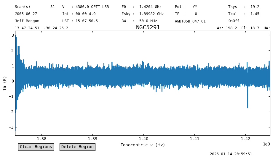
Get the time average of the calibrated data. This method returns a Spectrum.
ta = ps_scan_block.timeaverage()
ta.plot()
<dysh.plot.specplot.SpectrumPlot at 0x72de318ea0e0>
Reading and Writing Individual Spectra#
Inputs and Outputs#
dysh supports output to text files in a variety of formats familiar to users of astropy:
basic
commented_header
ECSV
fixed_width
IPAC
MRT
votable
The following lines of code define some of the available formats in a list, and then loop over them saving the calibrated data in each format.
We use the overwrite=True parameter to avoid errors if the files already exist on disk.
# Define the formats in a list.
fmt = [
    "basic",
    "commented_header",
    "ecsv",
    "fixed_width",
    "ipac",
    "mrt",
    "votable",
]

# Define the output directory and create it if it does not exists already.
output_dir = Path.cwd() / "output"
output_dir.mkdir(exist_ok=True)

# Loop over formats writing the calibrated spectrum.
for f in fmt:
    file = output_dir / f"testwrite.{f}"
    ta.write(file, format=f, overwrite=True)
We can also write a Spectrum to FITS format.
ta.write(output_dir / "testwrite.fits", format="fits", overwrite=True)
WARNING: Attribute `QD_XEL` of type <class 'float'> cannot be added to FITS Header - skipping [astropy.io.fits.convenience]
WARNING: Attribute `QD_EL` of type <class 'float'> cannot be added to FITS Header - skipping [astropy.io.fits.convenience]
WARNING: Attribute `TWARM` of type <class 'float'> cannot be added to FITS Header - skipping [astropy.io.fits.convenience]
WARNING: Attribute `TCOLD` of type <class 'float'> cannot be added to FITS Header - skipping [astropy.io.fits.convenience]
We can read spectra in FITS and a few formats. As noted in astropy, ECSV is the only ASCII format that can make a lossless output-input roundtrip and thus reproduce an original spectrum.
We use the Spectrum.read method to read the saved data.
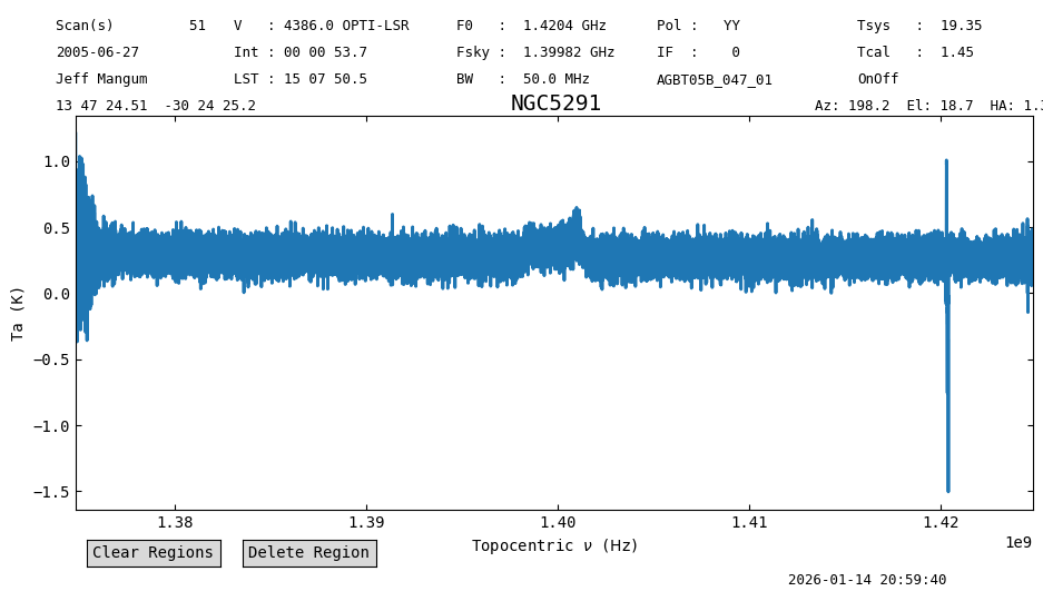
s1 = Spectrum.read(output_dir / "testwrite.fits", format="fits")
s1.plot()
<dysh.plot.specplot.SpectrumPlot at 0x72de31f0f610>

s2 = Spectrum.read(output_dir / "testwrite.ecsv", format="ecsv")
s2.plot()
<dysh.plot.specplot.SpectrumPlot at 0x72de260868c0>
GBTIDL ASCII format#
dysh can read text files created by GBTIDL’s write_ascii function. However, those files do not provide sufficient metadata to fully recreate the spectrum. (For instance, they do not have complete sky coordinate information.)
url = "https://www.gb.nrao.edu/dysh/example_data/onoff-L/gbtidl-data/onoff-L_gettp_156_intnum_0_HEL.ascii"
filename_ascii = from_url(url, savepath)
s3 = Spectrum.read(filename_ascii, format='gbtidl')
print(s3, "\n", s3.meta)
Spectrum (length=32768)
Flux=[3608710. 3553598. 3604808. ... 3523171. 3545982. 3474847.] ct,  mean=493422767.43425 ct
Spectral Axis=[1.42009237 1.42009166 1.42009094 ... 1.39665654 1.39665582
               1.39665511] GHz,  mean=1.40837 GHz
 {'SCAN': 156, 'OBJECT': 'NGC2782', 'DATE-OBS': '2021-02-10 00:00:00.000', 'RA': np.float64(119.42083333333332), 'VELDEF': 'None-HEL', 'POL': 'YY'}
dysh can even read compressed ASCII files. Note these data have velocity on the spectral axis.
url = "https://www.gb.nrao.edu/dysh/example_data/onoff-L/gbtidl-data/onoff-L_getps_152_RADI-HEL.ascii.gz"
filename_ascii_gz = from_url(url, savepath)
s4 = Spectrum.read(filename_ascii_gz, format='gbtidl')
print(s4, "\n", s4.meta)
Spectrum (length=32768)
Flux=[-0.1042543   0.05250004  0.00432693 ... -0.05038555  0.03408394
       0.06139921] K,  mean=0.17345 K
Spectral Axis=[1281.15245599 1281.30342637 1281.45439674 ... 6227.69690405
               6227.84787443 6227.99884481] km / s,  mean=3754.57565 km / s
 {'SCAN': 152, 'OBJECT': 'NGC2415', 'DATE-OBS': '2021-02-10 00:00:00.000', 'RA': np.float64(114.65624999999999), 'VELDEF': 'RADI-HEL', 'POL': 'YY'}
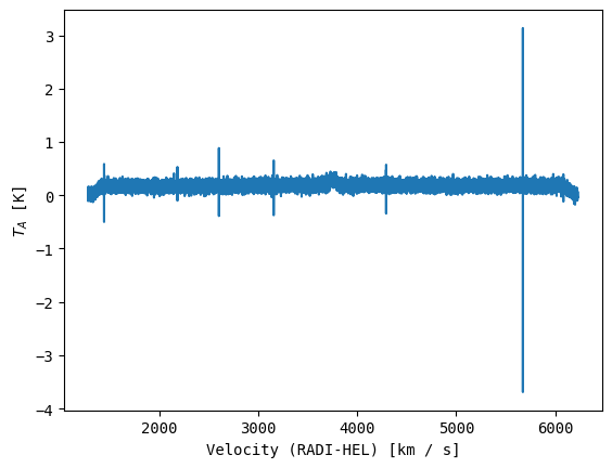
Plot#
To plot the spectrum contained in the ascii files you have to use matplotlib.
plt.figure()
plt.xlabel(f"Velocity ({s4.meta['VELDEF']}) [{s4.spectral_axis.unit}]")
plt.ylabel(f"$T_A$ [{s4.flux.unit}]")
plt.plot(s4.spectral_axis, s4.flux)
[<matplotlib.lines.Line2D at 0x72de25b9a500>]
Writing Multiple Calibrated Spectra to SDFITS#
You can write the calibrated data from a ScanBlock to the SDFITS format.
If there are multiple scans in the ScanBlock, they will all be written to the same SDFITS (useful for gbtgridder).
ps_scan_block.write(output_dir / "scanblock.fits", overwrite=True)
Reading Calibrated SDFITS#
To load the saved data, we use the same function we used to load the raw data, GBTFITSLoad.
ps_scan_block_read = GBTFITSLoad(output_dir / "scanblock.fits")
This is treated the same was as the raw data, so the same methods are available.
ps_scan_block_read.summary()
| SCAN | OBJECT | VELOCITY | PROC | PROCSEQN | RESTFREQ | DOPFREQ | # IF | # POL | # INT | # FEED | AZIMUTH | ELEVATION |
|---|---|---|---|---|---|---|---|---|---|---|---|---|
| 51 | NGC5291 | 4386.0 | OnOff | 1 | 1.420405 | 1.420405 | 1 | 1 | 11 | 1 | 198.3431 | 18.6427 |
However, since the data is already calibrated, trying to fetch the data using calibration methods like getps or getnod will result in errors.
Instead, we can use the gettp method or getspec.
Using gettp#
If we use gettp, then we will get all of the integrations as a ScanBlock object.
tp_read = ps_scan_block_read.gettp(scan=51, ifnum=0, plnum=0, fdnum=0)
print(f"Number of integrations: {tp_read[0].nint}")
Number of integrations: 11
We can access individual integration through the calibrated method.
ta_read_0a = tp_read[0].getspec(0)
ta_read_0a.plot()
<dysh.plot.specplot.SpectrumPlot at 0x72de25ba9750>

Using getspec#
Now we do the same using getspec. This method takes as input the row number we want to retrieve.
ta_read_0b = ps_scan_block_read.getspec(0)
ta_read_0b.plot()
<dysh.plot.specplot.SpectrumPlot at 0x72de2e22ccd0>
If we take the difference, it is zero.
(ta_read_0a.data - ta_read_0b.data).sum()
np.float64(0.0)
Writing Out Selected Data from GBTFITSLoad#
The write() method of GBTFITSLoad supports down-selection of data.
Data can be selected on any SDFITS column.
In the following call to GBTFITSLoad.write we will select a single polarization (plnum=1), and only the first five integrations of each scan (intnum=range(5)). We also set overwrite=True to avoid errors if the file already exists, and request that the output be saved into a single file (multifile=False).
sdfits.write(output_dir / "mydata.fits", plnum=1,
             intnum=range(5), overwrite=True, multifile=False)
 ID    TAG    PLNUM   INTNUM   # SELECTED
--- --------- ----- ---------- ----------
  0 0c0ae01cf     1 range(0,5)         80
These data, can of course, be read back in.
sdfits2 = GBTFITSLoad(output_dir / "mydata.fits")
sdfits2.summary()
| SCAN | OBJECT | VELOCITY | PROC | PROCSEQN | RESTFREQ | DOPFREQ | # IF | # POL | # INT | # FEED | AZIMUTH | ELEVATION |
|---|---|---|---|---|---|---|---|---|---|---|---|---|
| 51 | NGC5291 | 4386.0 | OnOff | 1 | 1.420405 | 1.420405 | 1 | 1 | 5 | 1 | 198.2327 | 18.6739 |
| 52 | NGC5291 | 4386.0 | OnOff | 2 | 1.420405 | 1.420405 | 1 | 1 | 5 | 1 | 198.8200 | 18.8193 |
| 53 | NGC5291 | 4386.0 | OnOff | 1 | 1.420405 | 1.420405 | 1 | 1 | 5 | 1 | 199.2207 | 18.3889 |
| 54 | NGC5291 | 4386.0 | OnOff | 2 | 1.420405 | 1.420405 | 1 | 1 | 5 | 1 | 199.8058 | 18.5264 |
| 55 | NGC5291 | 4386.0 | OnOff | 1 | 1.420405 | 1.420405 | 1 | 1 | 5 | 1 | 200.1952 | 18.0919 |
| 56 | NGC5291 | 4386.0 | OnOff | 2 | 1.420405 | 1.420405 | 1 | 1 | 5 | 1 | 200.7815 | 18.2213 |
| 57 | NGC5291 | 4386.0 | OnOff | 1 | 1.420405 | 1.420405 | 1 | 1 | 5 | 1 | 202.2201 | 17.4228 |
| 58 | NGC5291 | 4386.0 | OnOff | 2 | 1.420405 | 1.420405 | 1 | 1 | 5 | 1 | 202.8117 | 17.5334 |
Writing SDFITS to Multiple Files#
If the data came from multiple files, for instance VEGAS banks, then by default they are written to multiple files, so
sdfits.write('mydata.fits')
would write to mydata0.fits, mydata1.fits, … mydataN.fits.