Custom Baseline Fitting

dysh includes a baseline fitting method for its Spectrum objects, the baseline function. For simplicity, baseline uses astropy.modeling.polynomial as models. However, it is possible to fit any astropy.modeling.Model with some extra steps. Here we describe one possible approach.

Under the hood, the baseline method uses specutils.fitting.fit_continuum, which can take as input any astropy.modeling.Model. We can leverage this functionality to fit a custom model.

To illustrate this, we will create some fake data and then fit it.

Loading Modules

We start by loading the modules we will use to create the fake data and the baseline fit.

import numpy as np

from dysh.spectra import Spectrum
from specutils.fitting import fit_continuum
from astropy import modeling
from astropy import units as u

Make Fake Data

We create a Spectrum object. This would be the result of time averaging some calibrated data.

spectrum = Spectrum.fake_spectrum()

Next, we add a power law to it, to represent a type of model that is not one of astropy.modeling.polynomial models. We use a power law with an exponent, alpha, of -12.7 and an amplitude of 10 K at the first channel of the spectrum, x_0.

amplitude = 10 * u.K
alpha = -12.7
x_0 = spectrum.spectral_axis.quantity[0]
power_law_values = amplitude * np.power(spectrum.spectral_axis.quantity / x_0, alpha)

We add the power law to our spectrum. This will be our starting point for the fit.

spectrum += power_law_values

See how it looks.

plot = spectrum.plot(xaxis_unit="GHz")

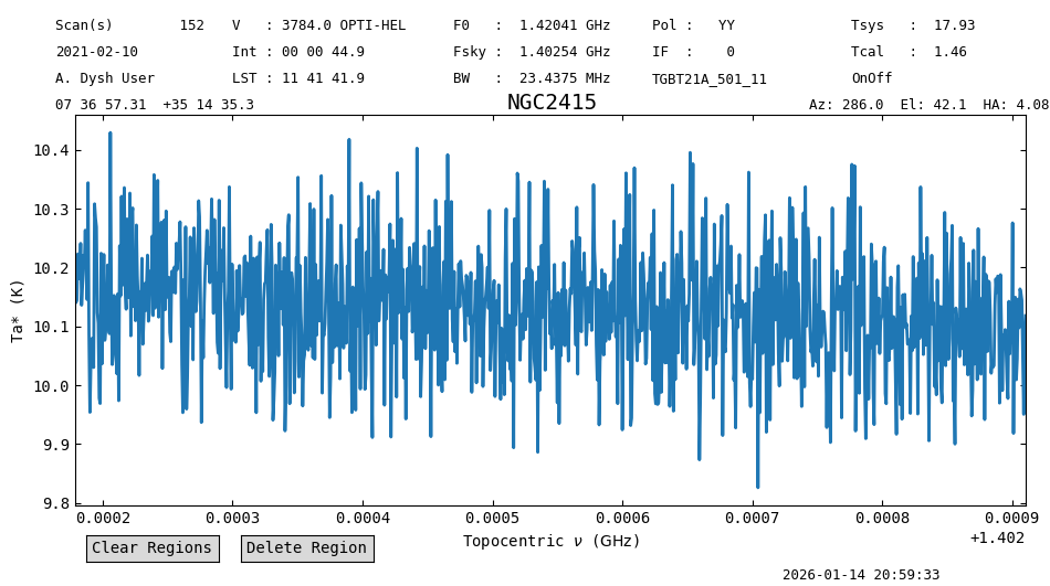
The power law is not obvious, as our spectrum only covers a small frequency range. But we know it is there, because the spectrum is offset from zero and it has a slope.

Custom Model Fitting

Now we define our model using astropy.modeling. When we define our model we must specify the starting guess for the model parameters. We will use starting values not too far from the answer.

model = modeling.powerlaws.PowerLaw1D(amplitude=5*u.K, 
                                      x_0=spectrum.spectral_axis.quantity[0],
                                      alpha=-10.)

Now, we use this model to fit our spectrum.

model_fit = fit_continuum(spectrum, model=model)

The return from fit_continuum is our model with the best fit parameters.

model_fit

<PowerLaw1D(amplitude=9.76794106 K, x_0=1.40697771e+09 Hz, alpha=11.5652202)>

Now, we evaluate the model over the same frequency range as our spectrum and plot it on top of the data. To add it to the plot we leverage the SpectrumPlot.axis attribute, which is the matplotlib.axes.Axes object that contains the plotted elements.

model_fit_values = model_fit(spectrum.spectral_axis)
plot.axis.plot(spectrum.spectral_axis, model_fit_values, label="Best fit model")
plot.axis.legend()
plot.figure

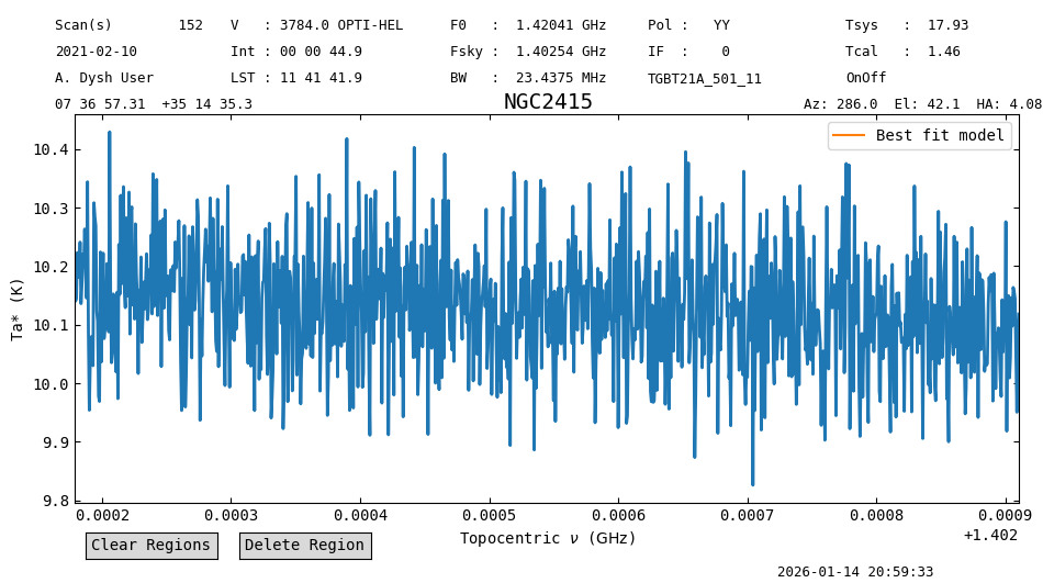
So, even if the best fit alpha was far from the input, this model still describes the fake data reasonably well.

Model Removal

We can remove this baseline model from the spectrum using arithmetic:

baseline_removed_spectrum = spectrum - model_fit_values
baseline_removed_spectrum.plot();

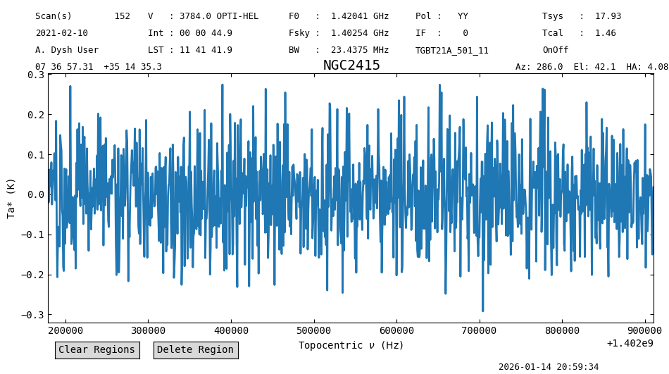
The baseline model has been removed from baseline_removed_spectrum, as the spectrum is now centered around zero.

Please check astropy.modeling for more models and additional options that can be used during the fitting.