On-The-Fly (OTF) Data Reduction#
This notebook shows how to use dysh to calibrate and grid an On-The-Fly (OTF) observation. See Mangum et al. (2007) for the background on this method.
OTF observations can be calibrated in dysh, however, generating FITS cubes requires the use of additional applications.
The workflow to go from raw data to a FITS cube would then require the following steps:
Calibrate the data using
dysh. This can include baseline subtraction, altough in some cases baseline removal is more effective in a FITS cube.Write the calibrated spectra to a format compatible with the gridding tool being used. For GBT observations the recommended format is SDFITS and the tool to grid the data is the gbtgridder.
Baseline subtraction in the FITS cube. This is optional, depending on the data quality, and
dyshdoes not provide convenience functions for this.
You can find a copy of this tutorial as a Jupyter notebook here or download it by right clicking here and selecting “Save Link As”.
Loading Modules#
We start by loading the modules we will use for the data reduction.
For display purposes, we use the static (non-interactive) matplotlib backend in this tutorial. However, you can tell matplotlib to use the ipympl backend to enable interactive plots. This is only needed if working on jupyter lab or notebook.
# We use dysh_data to retrieve the example data set.
from dysh.util.files import dysh_data

# This is required to load and calibrate the example data set.
from dysh.fits.gbtfitsload import GBTFITSLoad
Data Retrieval#
Download the example SDFITS data, if necessary.
# example="otf1" also works
filename = dysh_data(example='mapping-L/data/TGBT17A_506_11.raw.vegas/TGBT17A_506_11.raw.vegas.A.fits')
Downloading TGBT17A_506_11.raw.vegas.A.fits from http://www.gb.nrao.edu/dysh//example_data/mapping-L/data/TGBT17A_506_11.raw.vegas/TGBT17A_506_11.raw.vegas.A.fits
Retrieved TGBT17A_506_11.raw.vegas.A.fits
sdfits = GBTFITSLoad(filename)
sdfits.summary()
| SCAN | OBJECT | VELOCITY | PROC | PROCSEQN | RESTFREQ | DOPFREQ | # IF | # POL | # INT | # FEED | AZIMUTH | ELEVATION |
|---|---|---|---|---|---|---|---|---|---|---|---|---|
| 6 | 3C286 | 0.0 | OnOff | 1 | 1.6168 | 1.420406 | 5 | 2 | 13 | 1 | 248.3657 | 72.5531 |
| 7 | 3C286 | 0.0 | OnOff | 2 | 1.6168 | 1.420406 | 5 | 2 | 13 | 1 | 250.0385 | 73.6777 |
| 8 | SgrB2M | 57.0 | Track | 1 | 1.6168 | 1.420406 | 5 | 2 | 61 | 1 | 142.3845 | 12.2545 |
| 9 | W33B | 64.0 | Track | 1 | 1.6168 | 1.420406 | 5 | 2 | 61 | 1 | 132.2057 | 17.9786 |
| 10 | G30.589-0.044 | 38.0 | Track | 1 | 1.6168 | 1.420406 | 5 | 2 | 61 | 1 | 115.4811 | 25.5523 |
| 11 | G31.412+0.307 | 97.0 | Track | 1 | 1.6168 | 1.420406 | 5 | 2 | 61 | 1 | 115.8034 | 27.0986 |
| 12 | G35.577-0.029 | 49.0 | Track | 1 | 1.6168 | 1.420406 | 5 | 2 | 61 | 1 | 112.3139 | 29.0337 |
| 13 | G40.622-0.137 | 32.0 | Track | 1 | 1.6168 | 1.420406 | 5 | 2 | 61 | 1 | 107.7736 | 31.3159 |
| 14 | NGC6946 | 45.0 | DecLatMap | 1 | 1.6168 | 1.420406 | 5 | 2 | 61 | 1 | 38.9626 | 41.3644 |
| 15 | NGC6946 | 45.0 | DecLatMap | 2 | 1.6168 | 1.420406 | 5 | 2 | 61 | 1 | 38.9910 | 41.4488 |
| 16 | NGC6946 | 45.0 | DecLatMap | 3 | 1.6168 | 1.420406 | 5 | 2 | 61 | 1 | 38.9918 | 41.5360 |
| 17 | NGC6946 | 45.0 | DecLatMap | 4 | 1.6168 | 1.420406 | 5 | 2 | 61 | 1 | 39.0193 | 41.6203 |
| 18 | NGC6946 | 45.0 | DecLatMap | 5 | 1.6168 | 1.420406 | 5 | 2 | 61 | 1 | 39.0198 | 41.7075 |
| 19 | NGC6946 | 45.0 | DecLatMap | 6 | 1.6168 | 1.420406 | 5 | 2 | 61 | 1 | 39.0468 | 41.7919 |
| 20 | NGC6946 | 45.0 | DecLatMap | 7 | 1.6168 | 1.420406 | 5 | 2 | 61 | 1 | 39.0465 | 41.8791 |
| 21 | NGC6946 | 45.0 | DecLatMap | 8 | 1.6168 | 1.420406 | 5 | 2 | 61 | 1 | 39.0730 | 41.9637 |
| 22 | NGC6946 | 45.0 | DecLatMap | 9 | 1.6168 | 1.420406 | 5 | 2 | 61 | 1 | 39.0722 | 42.0508 |
| 23 | NGC6946 | 45.0 | DecLatMap | 10 | 1.6168 | 1.420406 | 5 | 2 | 61 | 1 | 39.0983 | 42.1355 |
| 24 | NGC6946 | 45.0 | DecLatMap | 11 | 1.6168 | 1.420406 | 5 | 2 | 61 | 1 | 39.0968 | 42.2227 |
| 25 | NGC6946 | 45.0 | DecLatMap | 12 | 1.6168 | 1.420406 | 5 | 2 | 61 | 1 | 39.1224 | 42.3073 |
| 26 | NGC6946 | 45.0 | DecLatMap | 13 | 1.6168 | 1.420406 | 5 | 2 | 61 | 1 | 39.1202 | 42.3945 |
| 27 | NGC6946 | 45.0 | Track | 1 | 1.6168 | 1.420406 | 5 | 2 | 61 | 1 | 39.0881 | 42.1493 |
In this particular observation the OTF slew over the galaxy NGC6946 in scans 14-26, followed by an Off position scan. Each SCAN, in this case, corresponds to a row, with 61 integrations as the telescope slews slowly over the sky.
Data Reduction#
We use getsigref to calibrate the OTF scans using scan 27 as the reference position.
getsigref takes as input a list of scan numbers, or a single one, and a number, or Spectrum, for the reference position.
It calibrates all the input scans using
We start by defining the variables we will use to calibrate the 21 cm-HI line observations present in this data set.
ifnum = 0                     # The 21 cm line is in the spectral window labeled 0.
fdnum = 0                     # Only one feed in this data set
ref   = 27                    # The reference ("OFF") scan
scans = list(range(14,27))    # The signal ("ON") scans
Now, we calibrate a single polarization. The processing for the second polarization should be almost identical.
sb0 = sdfits.getsigref(scan=scans, ref=ref, fdnum=fdnum, ifnum=ifnum, plnum=0)
The return from getsigref is a ScanBlock with PSScans in it.
sb0
ScanBlock([<dysh.spectra.scan.PSScan at 0x72eb219cdff0>,
           <dysh.spectra.scan.PSScan at 0x72ea8e89ace0>,
           <dysh.spectra.scan.PSScan at 0x72ea8e89bcd0>,
           <dysh.spectra.scan.PSScan at 0x72eb20a802e0>,
           <dysh.spectra.scan.PSScan at 0x72eb201e57b0>,
           <dysh.spectra.scan.PSScan at 0x72ea8ea200a0>,
           <dysh.spectra.scan.PSScan at 0x72ea8ea218a0>,
           <dysh.spectra.scan.PSScan at 0x72eb24313580>,
           <dysh.spectra.scan.PSScan at 0x72ea8e89acb0>,
           <dysh.spectra.scan.PSScan at 0x72ea8ea20670>,
           <dysh.spectra.scan.PSScan at 0x72ea8e89b520>,
           <dysh.spectra.scan.PSScan at 0x72ea8e89bc70>,
           <dysh.spectra.scan.PSScan at 0x72eb200b65c0>])
Data Inspection#
After calibrating the data, we can inspect the calibrated data using the plotting methods available in dysh.
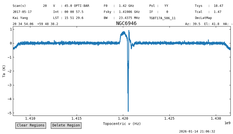
First, we will extract a single spectrum from the middle of the observations and plot it.
To get the spectrum from the middle of the OTF map, we use len(sb0)//2 to specify the middle scan and sb0[len(sb0)//2].nint//2 to specify the middle integration (in this case there are 61 integrations).
We store the number of integrations in the nint variable to reuse it later.
nint = sb0[len(sb0)//2].nint
spec = sb0[len(sb0)//2].getspec(nint//2)
sp = spec.plot()
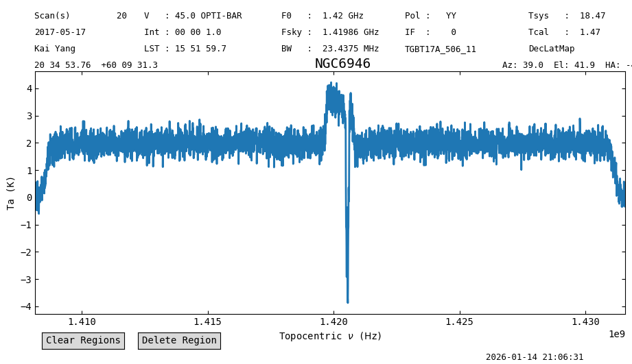
A clear and strong signal is present, as well as a ~2 K continuum.
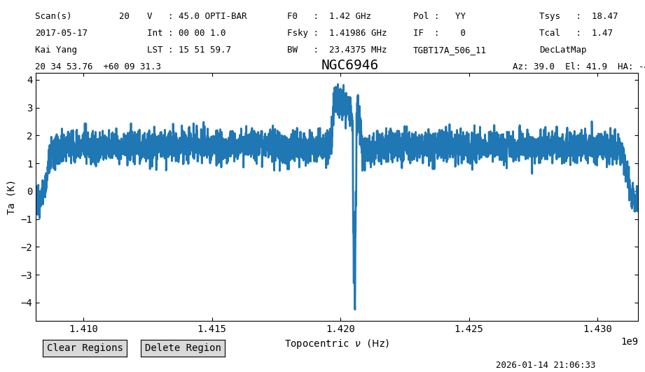
Now we will plot the time average for the middle scan.
spec_avg = sb0[len(sb0)//2].timeaverage()
sp_avg = spec_avg.plot()
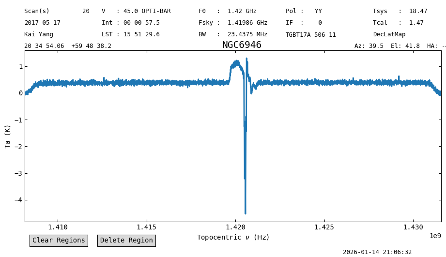
Again, a clear signal, but the line brightness and continuum are lower due to the dilution from the time averaging. This is because the source is smaller than the area mapped, so the signal gets averaged with empty sky.
Baseline Subtraction#
If we are only interested in the spectral line, then we use baseline subtraction to remove the continuum. We will use an order 1 polynomial to remove the continuum, and make sure to exclude the edge channels as well as the channels with 21 cm signal during the baseline fit.
We explore two approaches to continuum subtraction (baseline removal), using a model derived from a time average and deriving a baseline for each integration.
Using a Time Average#
We start by using the time average of the spectra in one scan to derive a baseline model, and then we will use this baseline model to subtract the continuum from all of the integrations in the scan. This approach has the benefit of being faster than deriving a baseline from each integration, and the spectrum used to derive the baseline model has a higher signal-to-noise. However, this approach requires that the baseline be stable in time/sky position. If that is not the case, then there will be left over baseline/continuum in the baseline subtracted data.
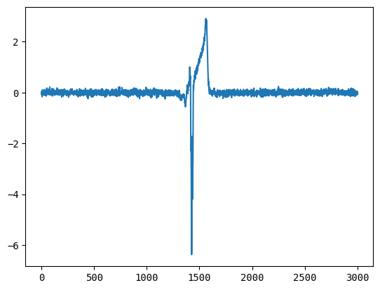
We start by plotting the time average as a function of channel number to determine where the 21 cm signal is.
sp_avg.plot(xaxis_unit="channel")
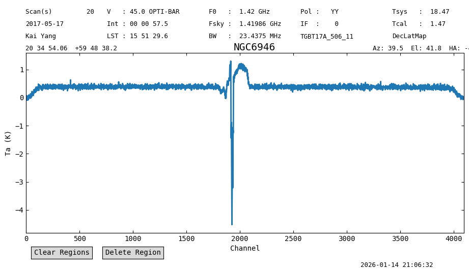
From the plot we see that channels ~1600 to 2250 have 21 cm signal, and the edges are between 0 and 250, and 4095-250 and 4095. We define an exclude region with these.
exclude = [(0,250),
           (1600,2250),
           (4095-250,4095)]
Now do the baseline fitting, using an order 1 polynomial and removing the best fit model from the data.
spec_avg.baseline(1, model="poly", exclude=exclude, remove=True)
Plot the baseline subtracted data.
(Alternatively, one could use spec_avg.plot().)
sp_avg.plot()
The continuum has been removed (the spectrum is centered around 0 K). We can look at the statistics to verify this.
spec_avg.stats()
{'mean': <Quantity -0.00863779 K>,
 'median': <Quantity -0.00468249 K>,
 'rms': <Quantity 0.25388794 K>,
 'min': <Quantity -4.90320558 K>,
 'max': <Quantity 0.91798011 K>,
 'npt': 4096,
 'nan': np.int64(2)}
The mean is around -8.6 mK, the median -4.5 mK and the rms 0.25 K.
We can subtract this baseline model from all of the integrations using the subtract_baseline method of a ScanBlock or Scan.
The input to subtract_baseline should be a baseline model, which can be accessed through the baseline_model attribute of a Spectrum object.
sb0[len(sb0)//2].subtract_baseline(spec_avg.baseline_model)
Generate a time average again to see how the data changed after the baseline subtraction.
spec_avg_bsub = sb0[len(sb0)//2].timeaverage()
sp_avg_bsub = spec_avg_bsub.plot()

The time average for the middle scan of the OTF map is now centered around zero as expected. However, since we used the diluted time average for the middle scan as our baseline model, the spectra that cover the source still have continuum left.
spec_bsub = sb0[len(sb0)//2].getspec(nint//2)
sp_spec_bsub = spec_bsub.plot()
Using the Integrations#
Now we will repeat the calibration, but deriving a baseline model from each integration. This is slower, so we only do this for the middle scan of the OTF map. This approach has the benefit of being more flexible than the previous one, however the signal-to-noise is worse.
To access the data for the integrations we will use the calibrated method and the _calibrated property of a Scan.
calibrated returns the data for a specific integration (starting at 0) as a Spectrum object, while _calibrated is the array that contains the calibrated data for the Scan.
We will use the Spectrum to derive the baseline, and then update the data by updating the _calibrated property of the Scan.
We put the middle scan of the OTF map in a new variable scan, then loop over its integrations fitting a baseline model and subtracting it from the calibrated data.
We ignore integrations that were blanked (all values would be NaN).
We use the math library to check for NaNs.
import math # Load the `math` library. Use this instead of `numpy` to save memory.
scan = sb0[len(sb0)//2]

for i,_c in enumerate(scan.calibrated):
    if math.isnan(_c.data.sum()):
        # If the sum is NaN, then skip (continue) this item.
        # This is not a great solution, as even a single NaN value
        # in the spectrum would cause the sum to be NaN,
        # but there should be no NaN values for single channels
        # in this data set.
        continue
    s_i = scan.getspec(i) # Fetch the `Spectrum` for integration `i`.
    s_i.baseline(1, model="poly", exclude=exclude, remove=True) # Fit a baseline model.
    scan.calibrated[i] -= s_i.baseline_model(s_i.spectral_axis).value # Subtract the baseline model from the data.
Plot the middle integration of the middle scan.
spec_bsub_int = sb0[len(sb0)//2].getspec(nint//2)
sp_spec_bsub_int = spec_bsub_int.plot()
Now the continuum has been removed.
We leave it as an exercise to repeat the above for every scan in the OTF map. The answer is hidden below.
Answer
            for i,_s in enumerate(sb0):
                for j,_c in enumerate(_s._calibrated):
                    if math.isnan(_c.data.sum()):
                        # If the sum is NaN, then skip (continue) this item.
                        continue
                    s_i = getspec(j)
                    s_i.baseline(1, model="poly", exclude=exclude, remove=True)
                    _s._calibrated[j] -= s_i.baseline_model(s_i.spectral_axis).value
This can be speed up if we only create a Spectrum once, and then update its data attribute with the data for each integration before computing the baseline. That would be:
            sp0 = sb0.timeaverage()
            for i,_s in enumerate(sb0):
                for j,_c in enumerate(_s._calibrated):
                    if math.isnan(_c.data.sum()):
                        # If the sum is NaN, then skip (continue) this item.
                        continue
                    sp0._data = _s._calibrated[j] # Update the data of the `Spectrum`.
                    sp0.baseline(1, model="poly", exclude=exclude, remove=True)
                    _s._calibrated[j] -= sp0.baseline_model(sp0.spectral_axis).value
Writing the Data#
After calibration, we write the data to disk in SDFITS format so it can be gridded by the gbtgridder (GBO’s supported data gridding tool).
sb0.write("otf_calibrated.fits", overwrite=True)
Gridding#
To grid GBT data GBO supports the use of the gbtgridder.
This is not included as part of dysh.
If you don’t have it installed, here’s a super short blurb how to get it, with the note that it is important to get the correct release branch.
git clone -b release_3.0  https://github.com/GreenBankObservatory/gbtgridder
cd gbtgridder
pip install .
This was the situation in the summer of 2025, and it may change, be sure to be in touch with the gbtgridder developers.
After installation, either from the shell, or from the notebook, one can grid as follows:
gbtgridder --size 32 32 --channels 500:3500 -o otf --auto otf_calibrated.fits
This is telling the gridder to produce an output cube with 32 by 32 pixels using only channels between 500 and 3500, and to use “otf” as the name of the output files. The --auto part is to skip a confirmation prompt. The last argument, otf_calibrated.fits, is the input SDFITS (which was created in the previous cell).
This call to the gbtgridder will create two files: otf_cube.fits and otf_weight.fits.
The first file contains the gridded data, and the second the weights used during the gridding process.
Working with Cubes#
dysh is not meant to work with image cubes, there are plenty of great tools for this.
Here we show how to use astropy to load the FITS cube and visualize its contents.
We use astropy.io.fits to load the data, astropy.wcs.WCS to generate a World Coordinate System (WCS) representation out of the FITS header, this is handy for plotting.
And, matplotlib.pyplot to plot.
from astropy.io import fits
from astropy.wcs import WCS
import matplotlib.pyplot as plt
Before proceeding we download the cube, in case you did not make your own.
Note that this cube was made using data which had the baseline subtracted using a per integration model. If you generate your own cubes, there might be differences with respect to the cube used here.
cube_filename = dysh_data(example='mapping-L/outputs/otf_cube.fits')
Downloading otf_cube.fits from http://www.gb.nrao.edu/dysh//example_data/mapping-L/outputs/otf_cube.fits
Retrieved otf_cube.fits
Open the FITS cube, extract the data and header and then create a WCS object.
with fits.open(cube_filename) as hdu:
    data = hdu[0].data
    head = hdu[0].header
wcs = WCS(head)
WARNING: FITSFixedWarning: 'datfix' made the change 'Set MJD-OBS to 57890.224583 from DATE-OBS'. [astropy.wcs.wcs]
The data object is an array with 4 dimensions, the first being the Stokes axis, the second the spectral axis, the third the latitude (e.g., Dec), and the fourth the longitude (e.g., RA). Altough the FITS cube has a Stokes axis, the gbtgridder does not handle polarizations properly, so if you have multiple polarizations in the input SDFITS file(s), the gbtgridder will average them.
To plot the spectrum from the center pixel we use.
plt.figure()
plt.plot(data[0,:,16,16])
[<matplotlib.lines.Line2D at 0x72ea8eb75a20>]
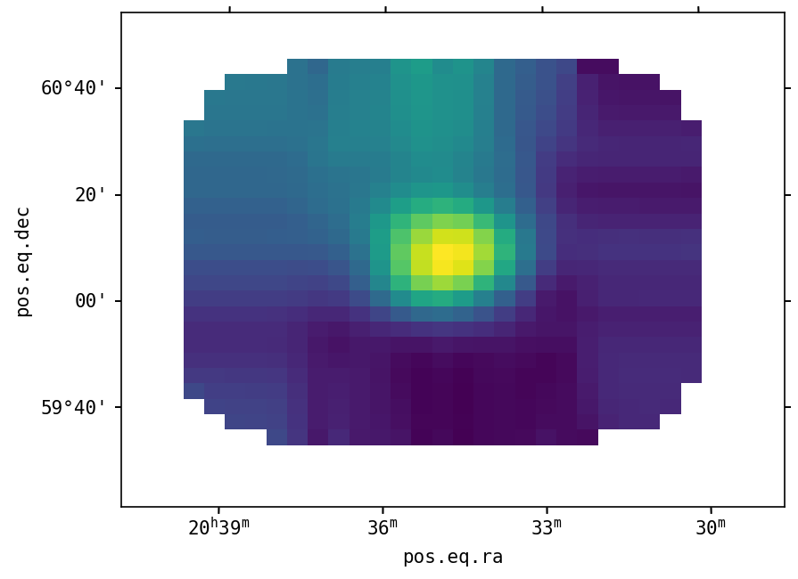
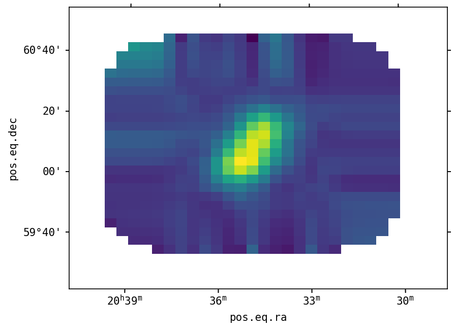
Now plot an image with the mean of the spectral axis.
We use the projection argument of fig.add_subplot to tell matplotlib to use the projection defined by the WCS object.
This takes care of using sky coordinates in the figure.
While plotting, imshow, we tell matplotlib to put the origin of the data, pixel (0,0), in the lower left corner (origin="lower"), and to automatically adjust the aspect ratio (aspect="auto") for the axes (not really needed since the data is already a square).
fig = plt.figure(dpi=150)
ax = fig.add_subplot(111, projection=wcs.celestial)
ax.imshow(data[0].mean(axis=0), origin="lower", aspect="auto")
<matplotlib.image.AxesImage at 0x72ea8b8c8d60>
Plot the data for channel 1500.
We use the celestial representation of the WCS object (wcs.celestial) to ignore the non celestial axes (e.g., Stokes and spectral).
fig = plt.figure(dpi=150)
ax = fig.add_subplot(111, projection=wcs.celestial)
ax.imshow(data[0,1500], origin="lower", aspect="auto")
<matplotlib.image.AxesImage at 0x72ea8b85f8e0>
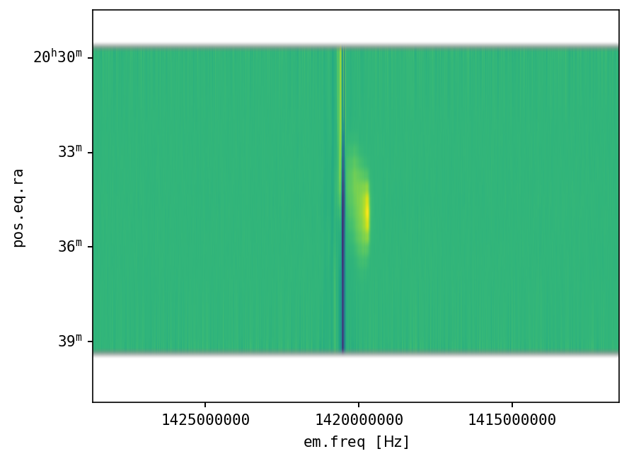
Plot a PV diagram.
Since we have multiple WCS axes (4), we use the slices argument, which tells the WCS object which axes to use for which axis. In this case the first WCS axis (longitude) goes in the y-axis of the figure, the latitude is fixed to its value at pixel 16, the third dimension (spectral axis) is shown in the x-axis, and the last dimensions (Stokes) is fixed to its value at pixel 0 (the only possibility in this case).
See these links for more details on how to use astropy for plotting cubes with multiple WCS axes: link1, and link2.
fig = plt.figure(dpi=150)
ax = fig.add_subplot(111, projection=wcs, slices=('y', 16, 'x', 0))
ax.imshow(data[0,:,:,16].T, origin="lower", aspect="auto")
<matplotlib.image.AxesImage at 0x72ea8b8cb730>