Gaussian Fitting#
This recipe shows how to use astropy and specutils to fit a Gaussian line profile to a Spectrum.
The data comes from the calseq tutorial.
You can find a copy of this tutorial as a Jupyter notebook here or download it by right clicking here and selecting “Save Link As”.
Loading Modules#
We start by loading the modules we will use for the data reduction.
For display purposes, we use the static (non-interactive) matplotlib backend in this tutorial. However, you can tell matplotlib to use the ipympl backend to enable interactive plots. This is only needed if working on jupyter lab or notebook.
# These are the modules we will use for loading the data and fitting.
from dysh.spectra import Spectrum
from specutils.fitting import fit_lines
from astropy.modeling import models
from astropy import units as u

# These modules are only used to download the data.
from pathlib import Path
from dysh.util.download import from_url
Data Retrieval#
Download the example FITS spectrum, if necessary.
url = "http://www.gb.nrao.edu/dysh/example_data/nod-W/outputs/M82_ifnum_3_polavg.fits"
savepath = Path.cwd() / "data"
savepath.mkdir(exist_ok=True) # Create the data directory if it does not exist.
filename = from_url(url, savepath)
Data Loading#
We use Spectrum.read to load the spectrum.
spec = Spectrum.read(filename, format="fits")
The loaded spectrum is now a Spectrum, with all its methods.
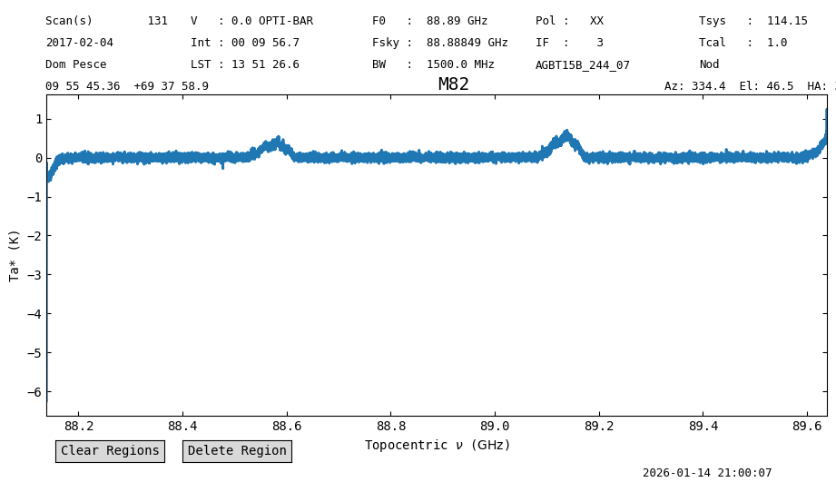
We can plot it, using Spectrum.plot.
sp_plt = spec.plot(xaxis_unit="GHz")
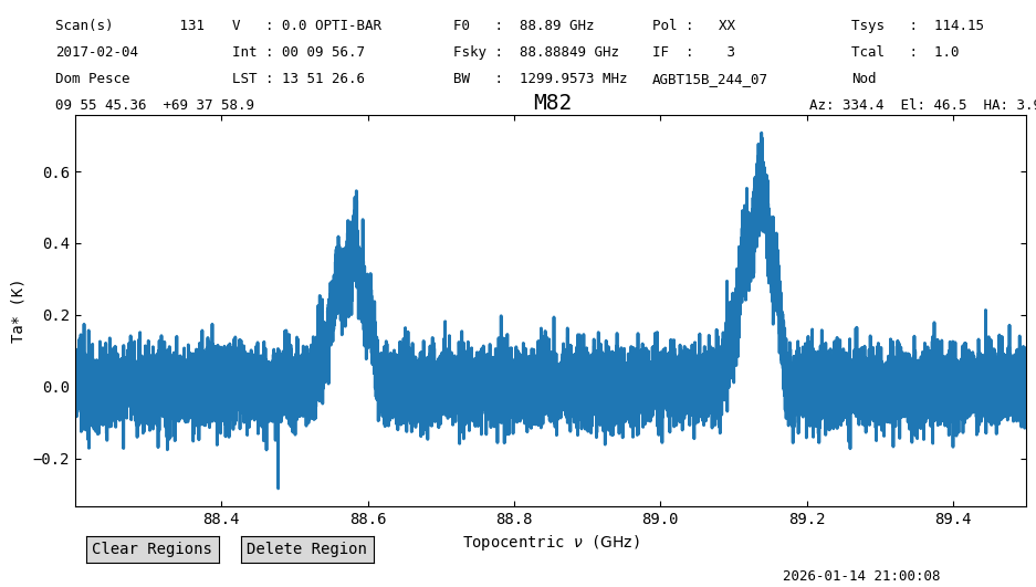
Before fitting, lets remove the edges of the spectrum. We only keep channels between 88.2 and 89.5 GHz.
spec = spec[88.2*u.GHz:89.5*u.GHz]
Plot again.
spec_plt = spec.plot(xaxis_unit="GHz")
Now we are ready to start fitting.
Gaussian Fitting#
Here we show how to fit a Gaussian profile using astropy and specutils.
There are other options available, but we won’t cover them all.
Fitting a Single Gaussian#
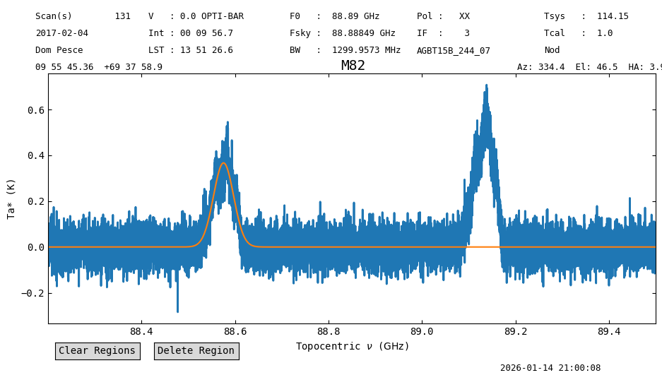
We start fitting a single Gaussian line profile to the line on the left, at about 88.55 GHz.
We create a model, with starting values, and then use the specutils.fitting.fit_lines function to fit the model to the spectrum.
After the fit is done, we evaluate the best fit model over the spectral axis of the spectrum so we can plot it on top of the data.
g_init = models.Gaussian1D(amplitude=0.5*u.K, mean=88.55*u.GHz, stddev=0.1*u.GHz)
g_fit = fit_lines(spec, g_init)
y_fit = g_fit(spec.spectral_axis)
Now plot it. We assign a “group id” (gid), so we can remove the line after.
spec_plt.axis.plot(spec.spectral_axis.to("GHz"), y_fit, gid="1gauss")
spec_plt.figure # This will show the figure here.
Extracting Best Fit Parameters#
The best fit parameters are now properties of the output best fit model. We can access them through the parameter names, for the Gaussian, amplitude, mean and stddev. For example, the line amplitude
g_fit.amplitude
Parameter('amplitude', value=0.3670704696308813, unit=K)
and its formal error
g_fit.amplitude.std
np.float64(0.006236258674343532)
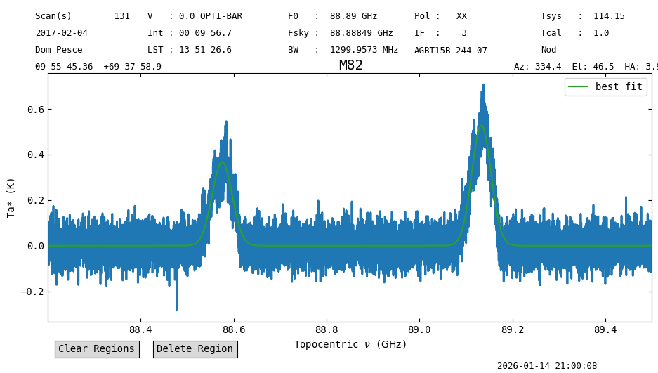
Fitting Two Gaussians#
We can also combine models. In this case, we add a second Gaussian line profile to fit the second line at about 89.15 GHz.
g_init2 = models.Gaussian1D(amplitude=0.6*u.K, mean=89.15*u.GHz, stddev=0.1*u.GHz)
g_fit = fit_lines(spec, g_init + g_init2)
y_fit = g_fit(spec.spectral_axis)
Before plotting the new model with two Gaussians, we remove the previous line.
spec_plt.clear_lines("1gauss")
We repeat the plotting with the new model results.
This time, we add a label to the best fit model line (label="best fit").
spec_plt.axis.plot(spec.spectral_axis.to("GHz"), y_fit, label="best fit")
spec_plt.axis.legend()
spec_plt.figure
You can find more examples of how to use specutils.fitting.fit_lines in the specutils documentation.
In the case of a compound model, the model parameters get assigned an underscore and a number to differentiate them.
So the amplitude of the first Gaussian is stored in g_fit.amplitude_0 and that of the second Gaussian in g_fit.amplitude_1
g_fit.amplitude_0
Parameter('amplitude', value=0.3670154759025372, unit=K)
g_fit.amplitude_1
Parameter('amplitude', value=0.5278759700867971, unit=K)
Other Profiles and Further Examples#
Additional profiles and models are available through the astropy.modeling submodule.
The astropy documentation also provides examples of how to fit models with constraints, and examples of how to fit models, without using specutils.