Work With Repeated Scan Numbers#
This recipe shows how to work with repeated scan numbers. It uses data from a RFI scan, a trimmed down version.
In this case there are two occurrences of scan 2.
The two used a different number of channels, so they end up in different binary tables.
We will use GBTFITSLoad.summary to determine how to uniquely identify them, and then GBTFITSLoad.gettp to retrieve the data.
Loading Modules#
We start by loading the modules we will use for the recipe.
# These modules are required for the data reduction.
from dysh.fits.gbtfitsload import GBTFITSLoad

# These modules are only used to download the data.
from pathlib import Path
from dysh.util.download import from_url
url = "http://www.gb.nrao.edu/dysh/example_data/repeated-scans/data/TRFI_090125_S1.raw.vegas/TRFI_090125_S1.raw.vegas.testtrim.fits"
savepath = Path.cwd() / "data"
savepath.mkdir(exist_ok=True) # Create the data directory if it does not exist.
filename = from_url(url, savepath)
Data Loading#
Next, we use GBTFITSLoad to load the data, and then its summary method to inspect its contents.
sdfits = GBTFITSLoad(filename)
sdfits.summary()
| SCAN | OBJECT | VELOCITY | PROC | PROCSEQN | RESTFREQ | DOPFREQ | # IF | # POL | # INT | # FEED | AZIMUTH | ELEVATION |
|---|---|---|---|---|---|---|---|---|---|---|---|---|
| 2 | rfiscan1 | 0.0 | Track | 1 | 2.15 | 2.15 | 1 | 1 | 4 | 1 | 15.3022 | 44.5177 |
| 2 | rfiscan2 | 0.0 | Track | 1 | 0.75 | 0.75 | 1 | 1 | 4 | 1 | 172.2867 | 44.5177 |
The summary tells us there are two instances of scan 2. How can we tell them apart?
Identifying Data#
By default summary will separate the information by scan number (SCAN), project ID (PROJID) and binary table (BINTABLE).
Since we see there are two occurrences of scan 2, it means one of those columns has different values for each of them.
We can show more columns by using the add_columns argument of summary to inspect their values.
sdfits.summary(add_columns="BINTABLE, PROJID")
| SCAN | OBJECT | VELOCITY | PROC | PROCSEQN | RESTFREQ | DOPFREQ | # IF | # POL | # INT | # FEED | AZIMUTH | ELEVATION | BINTABLE | PROJID |
|---|---|---|---|---|---|---|---|---|---|---|---|---|---|---|
| 2 | rfiscan1 | 0.0 | Track | 1 | 2.15 | 2.15 | 1 | 1 | 4 | 1 | 15.3022 | 44.5177 | 0 | TRFI_090125_S1 |
| 2 | rfiscan2 | 0.0 | Track | 1 | 0.75 | 0.75 | 1 | 1 | 4 | 1 | 172.2867 | 44.5177 | 1 | TRFI_090125_S1 |
This shows that the data have the same project ID, and different binary tables. We can use the BINTABLE column to uniquely identify the data. The first occurrence has BINATBLE 0 and the second 1. It is important to note that the BINTABLE column gets a value depending on the contents of the file at the time of loading, so its value is not absolute. If you were working with the full data set the BINTABLE values would be different.
Retrieving Data#
Now that we know how to identify the scans we can use this information to retrieve the data we want.
We pass the bintable keyword to gettp to get the data we want.
For the first occurrence of scan 2 we use
tpsb1 = sdfits.gettp(scan=2, ifnum=0, plnum=0, fdnum=0, bintable=0)
For the second occurrence we use
tpsb2 = sdfits.gettp(scan=2, ifnum=0, plnum=0, fdnum=0, bintable=1)
Now we plot the two together to show that they are indeed different.
tpsb1_plt = tpsb1.timeaverage().plot(oshow=tpsb2.timeaverage())
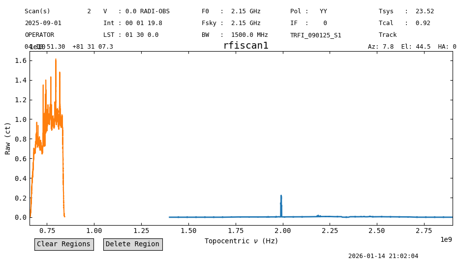
We can clearly see that they have different rest frequencies.