Modifying the Default Values for Surface Error and Aperture Efficiency#
We encourage users of the GBT to rely on the Observatory-measured values and functions for surface error and aperture efficiency, which are implemented in dysh. However, advanced users may wish to modify the values or functions; this example shows how to do that.
You can find a copy of this tutorial as a Jupyter notebook here or download it by right clicking here and selecting “Save Link As”.
Refresher on Aperture Efficiency and Brightness Scales#
The aperture efficiency \(\eta_a\) is determined by:
where \(\eta_0\) is the long wavelength aperture efficiency, \(G(ZD)\) is the gain correction factor at a zenith distance \(ZD\), \(\epsilon\) is the surface error, and \(\lambda\) is the wavelength.
To scale antenna temperature \(T_a\) to brightness tempeature \(T_a^*\):
where \(\tau\) is the zenith opacity, \(A\) is the airmass, and \(\eta_l\) is the loss efficiency. To scale to flux \(S_\nu\)
where \(k\) is Boltzmann’s constant is \(A_p\) is the physical aperture of the telescope.
What dysh Does#
When you calibrate and scale data through, e.g. GBTFITSLoad.getps, dysh uses the GBTGainCorrection class to manage the calculations described above. GBTGainCorrection maintains \(G(ZD)\) and surface error as a function of date as derived in GBT Memo 301. You can provide your own values for \(\eta_a\) or \(\epsilon\) in the standard calibration routines. (You must provide \(\tau\)).
Loading Modules#
We start by loading the modules we will use for the data reduction.
For display purposes, we use the static (non-interactive) matplotlib backend in this tutorial. However, you can tell matplotlib to use the ipympl backend to enable interactive plots. This is only needed if working on jupyter lab or notebook.
# Set interactive plots in jupyter.
#%matplotlib ipympl

# These modules are required for the data reduction.
from dysh.fits.gbtfitsload import GBTFITSLoad
from astropy import units as u
import numpy as np
from dysh.log import init_logging

# These modules are only used to download the data.
from pathlib import Path
from dysh.util.download import from_url
Set the logging level to INFO.
init_logging(2)
Data Retrieval#
Download the example SDFITS data, if necessary.
url = "http://www.gb.nrao.edu/dysh/example_data/positionswitch/data/AGBT05B_047_01/AGBT05B_047_01.raw.acs/AGBT05B_047_01.raw.acs.fits"
savepath = Path.cwd() / "data"
savepath.mkdir(exist_ok=True) # Create the data directory if it does not exist.
filename = from_url(url, savepath)
20:59:24.151 I Starting download...
20:59:25.098 I Saved AGBT05B_047_01.raw.acs.fits to /home/docs/checkouts/readthedocs.org/user_builds/dysh/checkouts/release-0.11.5/docs/source/how-tos/examples/data/AGBT05B_047_01.raw.acs.fits
Data Loading#
Next, we use GBTFITSLoad to load the data, and then its summary method to inspect its contents.
sdfits = GBTFITSLoad(filename)
sdfits.summary()
| SCAN | OBJECT | VELOCITY | PROC | PROCSEQN | RESTFREQ | DOPFREQ | # IF | # POL | # INT | # FEED | AZIMUTH | ELEVATION |
|---|---|---|---|---|---|---|---|---|---|---|---|---|
| 51 | NGC5291 | 4386.0 | OnOff | 1 | 1.420405 | 1.420405 | 1 | 2 | 11 | 1 | 198.3431 | 18.6427 |
| 52 | NGC5291 | 4386.0 | OnOff | 2 | 1.420405 | 1.420405 | 1 | 2 | 11 | 1 | 198.9306 | 18.7872 |
| 53 | NGC5291 | 4386.0 | OnOff | 1 | 1.420405 | 1.420405 | 1 | 2 | 11 | 1 | 199.3305 | 18.3561 |
| 54 | NGC5291 | 4386.0 | OnOff | 2 | 1.420405 | 1.420405 | 1 | 2 | 11 | 1 | 199.9157 | 18.4927 |
| 55 | NGC5291 | 4386.0 | OnOff | 1 | 1.420405 | 1.420405 | 1 | 2 | 11 | 1 | 200.3042 | 18.0575 |
| 56 | NGC5291 | 4386.0 | OnOff | 2 | 1.420405 | 1.420405 | 1 | 2 | 11 | 1 | 200.8906 | 18.1860 |
| 57 | NGC5291 | 4386.0 | OnOff | 1 | 1.420405 | 1.420405 | 1 | 2 | 11 | 1 | 202.3275 | 17.3853 |
| 58 | NGC5291 | 4386.0 | OnOff | 2 | 1.420405 | 1.420405 | 1 | 2 | 11 | 1 | 202.9192 | 17.4949 |
Data Reduction#
We calibrate a few scans of the position switched observations, giving a value for zenith_opacity but leaving dysh to calculate the aperture efficiency.
We will calibrate scans 51, 53 and 55.
We use a zenith opacity of 0.08, but the exact values is not important here.
And, we request that the data be calibrated to units of flux, so that the aperture efficiency goes into the calculations.
scans = [51,53,55]
ps_scan_block = sdfits.getps(scan=scans, ifnum=0, plnum=0, fdnum=0, units="flux",
                             zenith_opacity=0.08)
Providing Aperture Efficiency or Surface Error#
Now, we calibrate the same data, but we provide a value for the aperture efficiency.
We use a value of \(25\%\) (ap_eff=0.25).
ps_scan_block_ap_eff = sdfits.getps(scan=scans, ifnum=0, plnum=0, fdnum=0, units="flux",
                                    zenith_opacity=0.08, ap_eff=0.25)
Alternatively, one could specify the surface error using the surface_error argument.
The value of the surface_error must be a quantity with units compatible with a length.
(You can’t give both surface error and aperture efficiency because the latter is computed from the former.)
ps_scan_block_surf_err = sdfits.getps(scan=scans, ifnum=0, plnum=0, fdnum=0, units="flux",
                                      zenith_opacity=0.08, surface_error=400*u.micron)
Now we print the different \(\eta_a\) for the first scan in each ScanBlock.
You can see that at this wavelength, the surface error does not have much of an effect because \(\epsilon << \lambda\). (400 \(\mu\)m vs. 21 cm)
print(f"{np.mean(ps_scan_block[0].ap_eff):.4f},{np.mean(ps_scan_block_ap_eff[0].ap_eff):.4f},{np.mean(ps_scan_block_surf_err[0].ap_eff):.4f}")
0.7047,0.2500,0.7045
But the aperture efficiency does make a different in the derived flux.
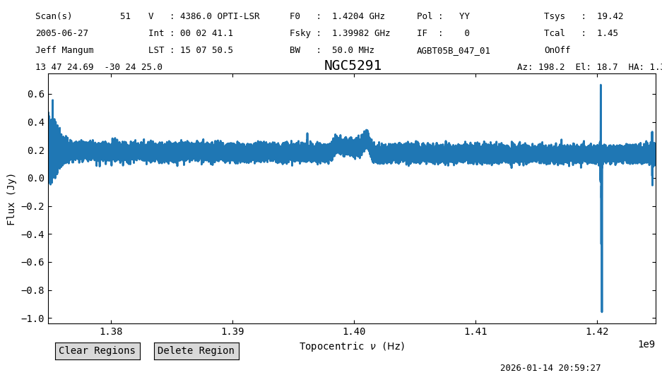
a = ps_scan_block.timeaverage()
print(f"S_nu = {a.stats()['median']:.3}")
a.plot()
S_nu = 0.18 Jy
<dysh.plot.specplot.SpectrumPlot at 0x74cded0ff130>
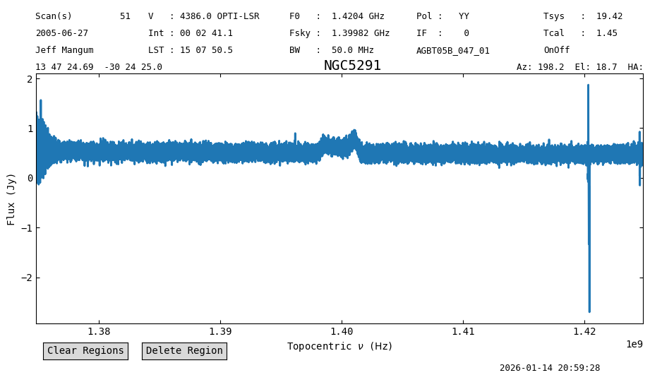
b = ps_scan_block_ap_eff.timeaverage()
print(f"S_nu = {b.stats()['median']:.3}")
b.plot()
S_nu = 0.508 Jy
<dysh.plot.specplot.SpectrumPlot at 0x74cdf46c9690>
The weighted average aperture efficiency, surface error, and zenith opacity are stored in the Spectrum metadata.
print(f"eta = {a.meta['AP_EFF']:.3f}, epsilon = {a.meta['SURF_ERR']:.1f} {a.meta['SE_UNIT']}, tau = {a.meta['TAU_Z']:.2f}")
eta = 0.705, epsilon = 230.0 micron, tau = 0.08
What if I want to change \(G(ZD)\) or the surface error model?#
This is advanced usage and requires you to fork or clone dysh, then modify src/dysh/data/gaincorrection.tab. If you have questions, consult with a dysh developer.