dysh Interactive Plotter Tutorial

In this tutorial, we will walk through the features of the interactive plotter offered by dysh. First, we download data from an HI survey and open it with dysh.

from dysh.fits.gbtfitsload import GBTFITSLoad
from pathlib import Path
from dysh.util.download import from_url

url = "http://www.gb.nrao.edu/dysh/example_data/rfi-L/data/AGBT17A_404_01.raw.vegas/AGBT17A_404_01.raw.vegas.A.fits"
savepath = Path.cwd() / "data"
filename = from_url(url, savepath)
sdfits = GBTFITSLoad(filename)

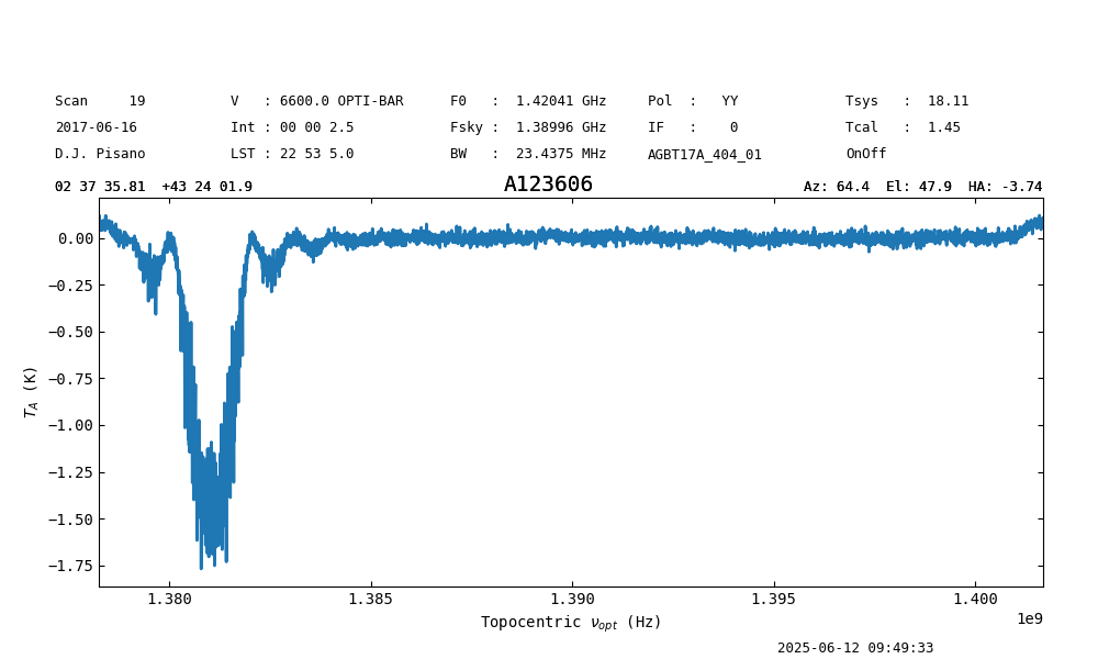
Now grab a position-switched scan with GPS interference, average it, and smooth with a 7-channel wide boxcar kernel. Start the interactive plotter with the plot() command. Spectrum.plot` supports a subset of the arguments offered by matplotlib.pyplot.plot. These are: xmin, xmax, ymin, ymax, xlabel, ylabel, xaxis_unit, yaxis_unit, grid, linewidth, color, and title. If you do not wish to have the interactive plotter and prefer a static plot, add interactive=False to the arguments.

ps = sdfits.getps(scan=19, plnum=0, fdnum=0, ifnum=0).timeaverage()
ps.plot()

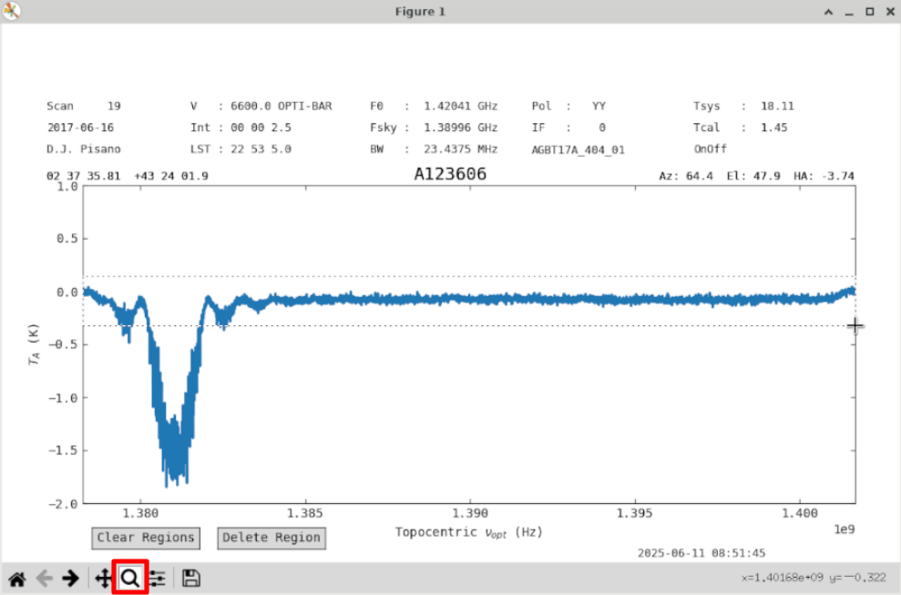
Use the matplotlib Zoom button (red) to Zoom into the baseline.

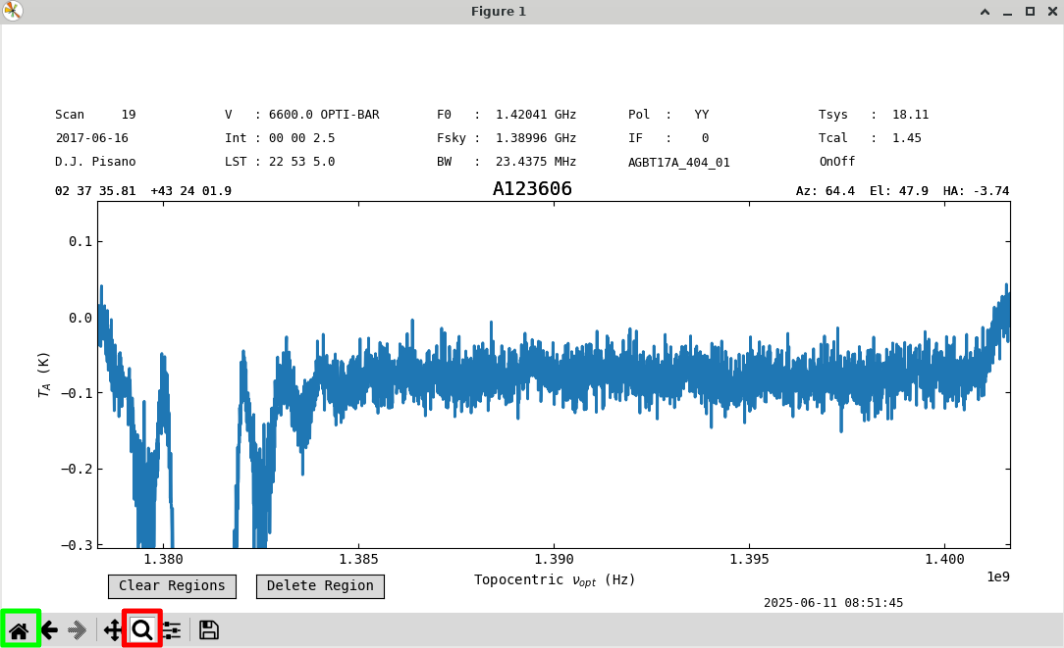
We will use a first order baseline. Uncheck the Zoom button (red) to re-enable region selection, and go back to the original zoom level with the Home button (green).

Create a region over the clean part of the spectrum by holding down left-click with your mouse and dragging across the screen.

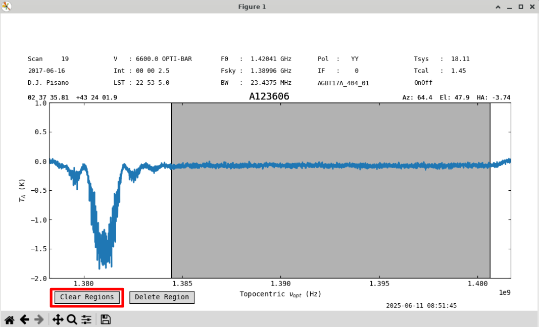
You can clear all regions with the “Clear Regions” (red) button.

You can click on a region to select it, allowing you to drag it to a different place in the spectrum or change its size. Currently, regions can only be resized by clicking near the edge from within the region. Regions are allowed to overlap. Once a region is selected, you can delete it with the “Delete Region” button.

Note

All buttons on the plot will disappear when using the ps.savefig() command. However, they will still remain in screenshots.

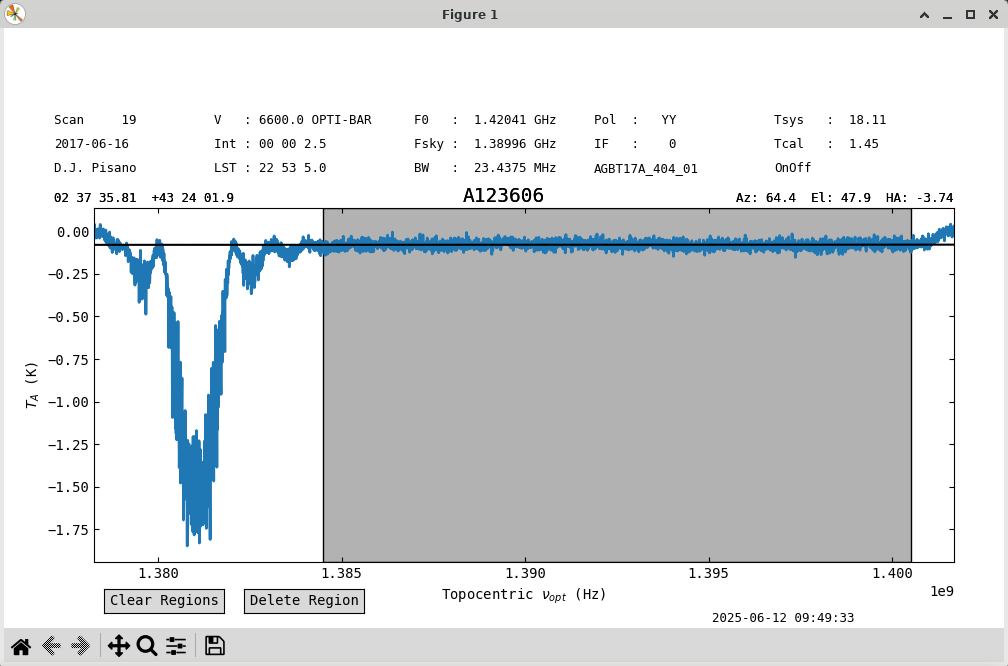
With one large region selected, we can try a baseline. Use the remove=False option to just plot the baseline fit without removing it.

ps.baseline(1,include=ps.get_selected_regions(),remove=False)

The fit looks good. Let’s subtract it out and save the figure. See that the buttons have disappeared. The white space at the top is reserved for buttons that will be implemented in the future and will be addressed. We can check the stats before and after to see they’ve improved.

ps.get_selected_regions()
[(210,2871)]

print(f"{ps[210:2871].stats()['mean']:.4f}, {ps[210:2871].stats()['rms']:.4f}")
-0.0780 K, 0.0204 K

ps.baseline(1,include=ps.get_selected_regions(),remove=True)

print(f"{ps[210:2871].stats()['mean']:.4f}, {ps[210:2871].stats()['rms']:.4f}")
-0.0000 K, 0.0204 K

ps.savefig('my_spectrum.png')