SubBeamNod Data Reduction#
This notebook shows how to use dysh to calibrate an SubBeamNod observation via two different methods. It retrieves and calibrates SubBeamNod scans using GBTFITSLoad.subbeamnod() which returns a ScanBlock object.
You can find a copy of this tutorial as a Jupyter notebook here or download it by right clicking here and selecting “Save Link As”.
Loading Modules#
We start by loading the modules we will use for the data reduction.
For display purposes, we use the static (non-interactive) matplotlib backend in this tutorial. However, you can tell matplotlib to use the ipympl backend to enable interactive plots. This is only needed if working on jupyter lab or notebook.
# Set interactive plots in jupyter.
#%matplotlib ipympl

# These modules are required for working with the data.
from dysh.fits.gbtfitsload import GBTFITSLoad

# These modules are only used to download the data.
from pathlib import Path
from dysh.util.download import from_url
Data Retrieval#
Download the example SDFITS data, if necessary.
url = "http://www.gb.nrao.edu/dysh/example_data/subbeamnod/data/AGBT13A_124_06/AGBT13A_124_06.raw.acs/AGBT13A_124_06.raw.acs.fits"
savepath = Path.cwd() / "data"
savepath.mkdir(exist_ok=True) # Create the data directory if it does not exist.
filename = from_url(url, savepath)
Data Loading#
Next, we use GBTFITSLoad to load the data, and then its summary method to inspect its contents.
sdfits = GBTFITSLoad(filename)
The returned sdfits can be probed for information.
You can also print a concise (or verbose if you choose verbose=True) summary of the data.
sdfits.summary()
| SCAN | OBJECT | VELOCITY | PROC | PROCSEQN | RESTFREQ | DOPFREQ | # IF | # POL | # INT | # FEED | AZIMUTH | ELEVATION |
|---|---|---|---|---|---|---|---|---|---|---|---|---|
| 44 | vIIzw31 | 16090.0 | SubBeamNod | 1 | 48.940955 | 48.990955 | 2 | 2 | 100 | 2 | 353.8967 | 47.7582 |
There is only one scan, using SubBeamNod. The scan is 44.
Data Reduction#
Single Scan#
To retrieve and calibrate a SubBeamNod scan we use sdfits.subbeamnod(). This method returns a ScanBlock, with one element per scan and per intermediate frequency.
Calibration per Cycle#
There are two different methods for calibrating a SubBeamNod scan. The first, with method="cycle" (the default) averages the data in each subreflector state for each cycle of integrations. That is, it separates the data into one signal/reference pair for each pair of subreflector states (on source and off source). Then calibrates each signal/reference pair independently and finally time averages the calibrated spectra.
sbn_scan_block = sdfits.subbeamnod(scan=44, fdnum=1, ifnum=0, plnum=0, method='cycle')
Time Averaging#
To time average the contents of a ScanBlock use its timeaverage method. Be aware that time averging will not check if the source is the same.
By default time averaging uses the following weights:
dysh these are set using weights='tsys' (the default).
ta = sbn_scan_block.timeaverage()
Plotting#
Plot the data and use different units for the spectral axis.
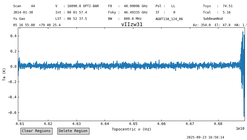
ta.plot()
<dysh.plot.specplot.SpectrumPlot at 0x74098326e170>
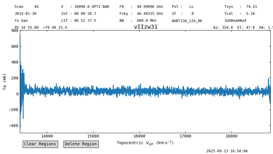
ta.plot(xaxis_unit="km/s", yaxis_unit="mK", ymin=-100, ymax=200)
<dysh.plot.specplot.SpectrumPlot at 0x74098326e170>
Calibration per Scan#
The second method (method="scan") of calibrating SubBeamNod scans reproduces the method of GBTIDL’s snodka.pro. This method treats the entire group of integrations as one cycle. It first time averages all of the integrations on source and off source, and then calibrates using the time averages.
sbn_scan_block2 = sdfits.subbeamnod(scan=44, fdnum=1, ifnum=0, plnum=0, method='scan')
ta2 = sbn_scan_block2.timeaverage()
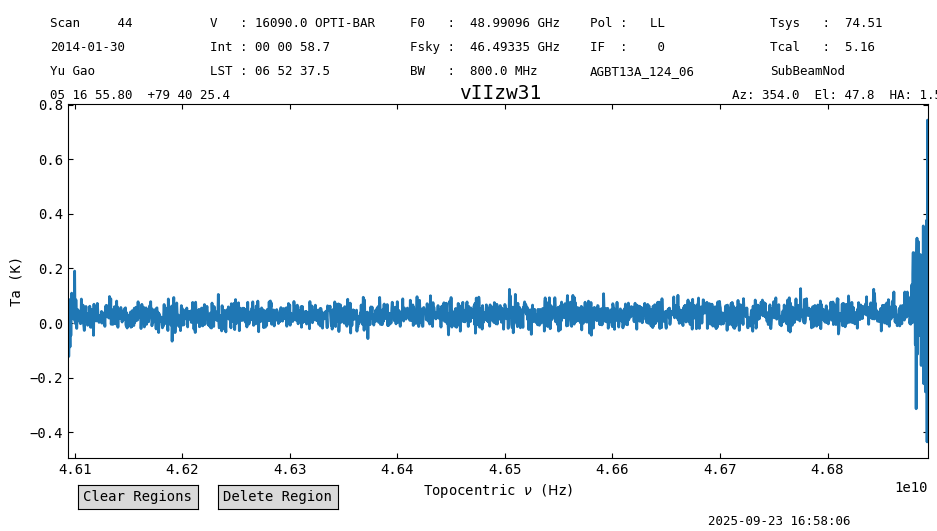
ta2.plot()
<dysh.plot.specplot.SpectrumPlot at 0x7409829cbd30>

Compare the Two Methods#
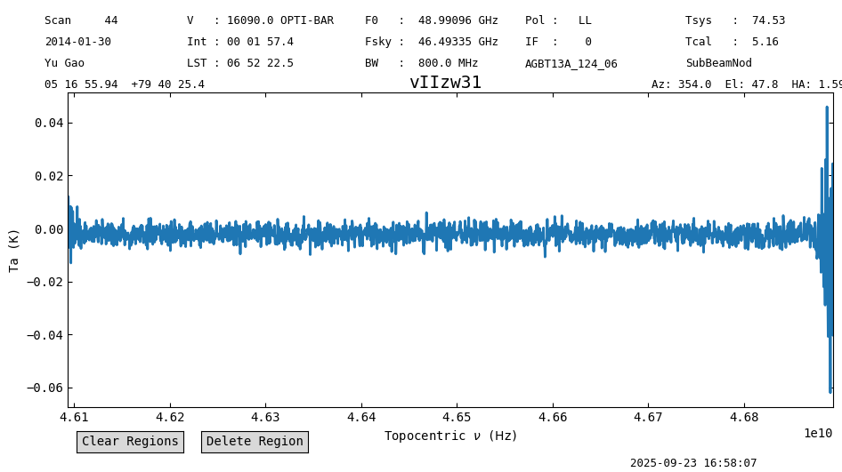
(ta2 - ta).plot()
<dysh.plot.specplot.SpectrumPlot at 0x7409828f7850>
Using Selection#
We will repeat the calibration but using selection. First we pre-select the data to be calibrated using the sdfits.select() method.
sdfits.select(scan=44)
sdfits.selection.show()
 ID    TAG    SCAN # SELECTED
--- --------- ---- ----------
  0 427fde300   44       1600
After using selection, the calibration routines will only look for data matching the selection rules. It is also possible to add additional rules for a specific calibration, like the polarization number.
sbn_scan_block3 = sdfits.subbeamnod(plnum=0, fdnum=1, ifnum=0)
ta3 = sbn_scan_block3.timeaverage()
ta3.plot()
<dysh.plot.specplot.SpectrumPlot at 0x74098326fd60>

Polarization Average#
Now we will calibrate the other polarization and average the two polarizations together.
First we calibrate the second polarization, then time average it and finally we average them together.
sbn_scan_block4 = sdfits.subbeamnod(plnum=1, fdnum=0, ifnum=0)
ta4 = sbn_scan_block4.timeaverage()
pol_avg = 0.5*(ta3 + ta4)
pol_avg.plot()
<dysh.plot.specplot.SpectrumPlot at 0x740983360550>