Flagging#
This guide shows how to use flags in dysh.
You can find a copy of this tutorial as a Jupyter notebook here or download it by right clicking here and selecting “Save Link As”.
Loading Modules#
We start by loading the modules we will use for this example.
For display purposes, we use the static (non-interactive) matplotlib backend in this tutorial. However, you can tell matplotlib to use the ipympl backend to enable interactive plots. This is only needed if working on jupyter lab or notebook.
# Set interactive plots in jupyter.
#%matplotlib ipympl

# We will use matplotlib for plotting.
import matplotlib.pyplot as plt

# These modules are required for working with the data.
from dysh.fits.gbtfitsload import GBTFITSLoad
from dysh.util.selection import Selection
import numpy as np

# These modules are only used to download and unpack the data.
import tarfile
from pathlib import Path
from dysh.util.download import from_url
Data Retrieval#
We download the data from a tar.gz file and then unpack it.
url = "http://www.gb.nrao.edu/dysh/example_data/rfi-L/data/AGBT17A_404_01.tar.gz"
savepath = Path.cwd() / "data"
savepath.mkdir(exist_ok=True) # Create the data directory if it does not exist.
filename = from_url(url, savepath)
# Unpack.
with tarfile.open(filename) as targz:
    targz.extractall('./data/')
    targz.close()
Data Loading#
After unpacking the data we load it. Notice how dysh tells us that it found a flag file.
sdfits = GBTFITSLoad("./data/AGBT17A_404_01.raw.vegas")
Flags were created from existing flag files. Use GBTFITSLoad.flags.show() to see them.
What flags were loaded?
sdfits.flags.show()
 ID TAG OBJECT BANDWID DATE-OBS ... SUBOBSMODE FITSINDEX CHAN UTC # SELECTED
--- --- ------ ------- -------- ... ---------- --------- ---- --- ----------
The above shows that the flag file was empty, so no flags were loaded.
Now, lets look at the summary.
sdfits.summary()
| SCAN | OBJECT | VELOCITY | PROC | PROCSEQN | RESTFREQ | DOPFREQ | # IF | # POL | # INT | # FEED | AZIMUTH | ELEVATION |
|---|---|---|---|---|---|---|---|---|---|---|---|---|
| 19 | A123606 | 6600.0 | OnOff | 1 | 1.420406 | 1.420406 | 1 | 2 | 61 | 1 | 64.5805 | 48.3795 |
| 20 | A123606 | 6600.0 | OnOff | 2 | 1.420406 | 1.420406 | 1 | 2 | 61 | 1 | 64.6012 | 48.4338 |
Data Inspection#
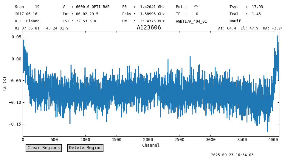
There are two scans, a pair of position switched observations. We will calibrate it and see how the data looks like.
We start by looking at the time average of the calibrated data.
# Calibrate the data.
ps_scanblock = sdfits.getps(scan=19, plnum=0, ifnum=0, fdnum=0)
# Compute the time average.
ps = ps_scanblock.timeaverage()
# Plot.
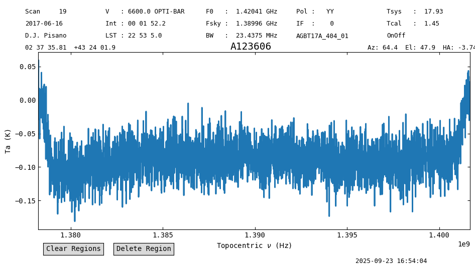
ps.plot(xaxis_unit="chan")
<dysh.plot.specplot.SpectrumPlot at 0x72bc223847f0>
There is radio frequency interference (RFI) for channels above ~2300. We will plot a waterfall to see if the RFI is confined in time.
This is done using the plot method of a ScanBlock.
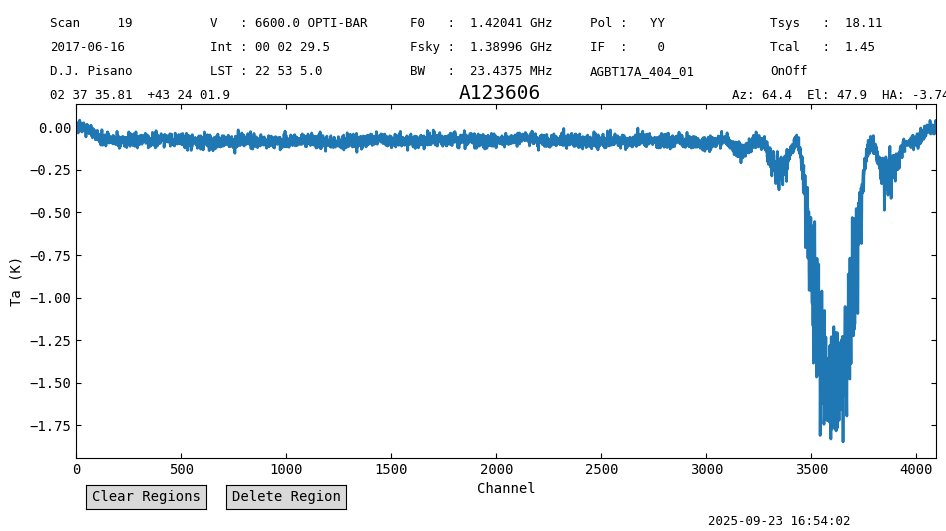
psp = ps_scanblock.plot()
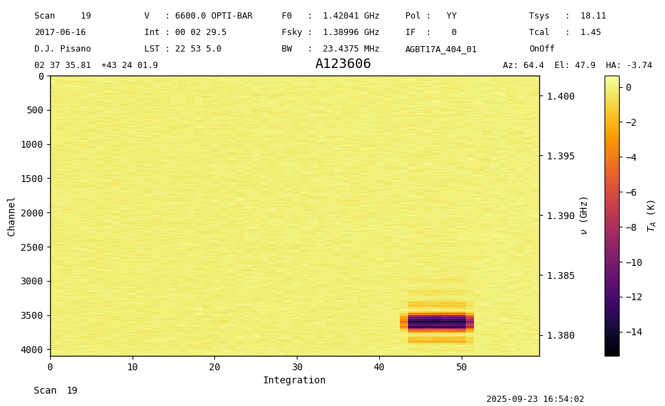
The RFI is confined to integrations 42 to 52, and it affects channels >2300. We will flag this range. Since the RFI shows as negative, it is also likely that this is present in the off scan, scan=20.
Data Flagging#
We use the GBTFITSLoad.flag method to generate flags.
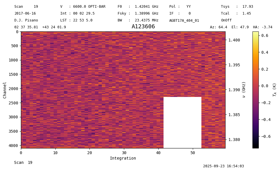
sdfits.flags.clear()
sdfits.flag(scan=20,
            channel=[[2300,4096]],
            intnum=[i for i in range(42,53)])
sdfits.flags.show()
 ID    TAG    SCAN              INTNUM                   CHAN     # SELECTED
--- --------- ---- -------------------------------- ------------- ----------
  0 36a177ecd   20 [42,43,44,45,46...8,49,50,51,52] [[2300,4096]]         44
We repeat the calibration after generating the flags.
pssb = sdfits.getps(scan=19, plnum=0, fdnum=0, ifnum=0, apply_flags=True)

pssb.plot()
<dysh.plot.scanplot.ScanPlot at 0x72bc1a0147c0>
The channels and times affected by RFI have been flagged. We can time average to generate the final spectrum without the RFI.
ps = pssb.timeaverage()
ps.plot(xaxis_unit="chan")
<dysh.plot.specplot.SpectrumPlot at 0x72bc193e3cd0>
Removing Flags#
To remove flags from the GBTFITSLoad object use the clear_flags method.
sdfits.clear_flags()
sdfits.flags.show()
 ID TAG OBJECT BANDWID DATE-OBS ... SUBOBSMODE FITSINDEX CHAN UTC # SELECTED
--- --- ------ ------- -------- ... ---------- --------- ---- --- ----------
Statistics-based Flagging#
We can assume that any significant increase in the standard deviation of the raw spectra is due to heavy RFI. Below, we will calculate mu + 3*sigma for each of the 8 individual switching states, and flag any integrations breaching that threshold.
The last integration has been blanked by VEGAS, and is not plotted below.
#Get raw spectra and standard deviations
specs = sdfits.rawspectra(0,0)
stdevs = np.std(specs,axis=1)


#Organize into scan and switching state.
#There are 2 scans for the target and reference pointings, 2 calibration diode states, and 2 polarizations.
stdevs = np.reshape(stdevs, (2,-1,4))

nrows = stdevs.shape[1]

#Inspect the data
for scan in range(2):
    for sw_state in range(4):
        plt.plot(stdevs[scan,:-1,sw_state],label=f'State {(4*scan)+sw_state}')

plt.xlabel('Integration #')
plt.ylabel('sigma')
plt.legend()
<matplotlib.legend.Legend at 0x72bc2135b0d0>
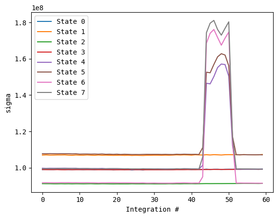
We can see that the 4 states corresponding to the OFF scan have a significant jump corresponding to the GPS L3 RFI. It does not appear to start until the 40th integration, so we will use that as our cutoff to calculate the statistics of the good data, and the thresholds to flag by.
flag_mask = np.zeros(stdevs.shape)
cutoff = 40

mean = np.mean(stdevs[:,:cutoff,:],axis=1)
spread = 3 * np.std(stdevs[:,:cutoff,:],axis=1)
Now we create our flagging mask of zeros and ones, where a one corresponds to a flag to be applied.
flag_mask = np.zeros(stdevs.shape)

mean = np.expand_dims(mean,axis=1)
spread = np.expand_dims(spread,axis=1)

flag_mask[stdevs > mean+spread] = 1
flag_mask = flag_mask.flatten()

flag_rows = np.where(flag_mask==1)[0].tolist()
print(flag_rows)
[176, 178, 185, 186, 187, 190, 191, 194, 195, 198, 199, 201, 202, 203, 206, 207, 208, 209, 210, 211, 214, 215, 216, 217, 218, 219, 222, 223, 226, 227, 230, 231, 234, 235, 236, 237, 238, 239, 240, 242, 416, 417, 418, 419, 420, 421, 422, 423, 424, 425, 426, 427, 428, 429, 430, 431, 432, 433, 434, 435, 436, 437, 438, 439, 440, 441, 442, 443, 444, 445, 446, 447, 448, 449, 450, 451, 484, 486]
We apply the flags using the “row” keyword, and see that the RFI is removed, along with a drop in the exposure time to 112 seconds instead of the original 150.
sdfits.flag(row=flag_rows)


ps = sdfits.getps(plnum=0, ifnum=0, fdnum=0).timeaverage()
print(ps.meta['EXPOSURE'])

ps.plot()
112.15101951854204
<dysh.plot.specplot.SpectrumPlot at 0x72bc1a01f7c0>