Quickstart Guide#
dysh is a Python spectral line data reduction and analysis program for single dish data with specific emphasis on data from the Green Bank Telescope. It is currently under development in collaboration between the Green Bank Observatory and the Laboratory for Millimeter-Wave Astronomy (LMA) at the University of Maryland (UMD). It is intended to replace GBTIDL, GBO’s current spectral line data reduction package.
Below is a “quickstart” guide with the essentials. A deeper dive into dysh’s capablities can be found in the Users Guide.
Installation#
Directly from github:
pip install "dysh[nb] @ git+https://github.com/GreenBankObservatory/dysh"
Latest stable release on PyPI:
pip install dysh[nb]
Read on for a brief overview.
Tip
You can find detailed installation instructions in Installing dysh.
Launching dysh#
After being installed, the dysh command will be available through the command line.
This will launch an iPython session with some modules and classes pre-loaded (e.g., GBTFITSLoad), and with logging.
We refer to this interface as the dysh shell.
Loading Data#
dysh can read and write SDFITS files.
Once inside the dysh shell loading an SDFITS file can be done using GBTFITSLoad.
The following lines of code will download an SDFITS, and then open it using GBTFITSLoad.
Downloading this data set is only required to follow this quick start as is.
# The following line will download 31 MB to the current working directory.
filename = dysh_data(example="getfs2")
sdfits = GBTFITSLoad(filename) # This will load the SDFITS file(s) at `filename`.
In the above code, you can replace filename with a path to your own data.
Either a single SDFITS file or a directory containing multiple SDFITS files will work.
The contents of the loaded data can be inspected using the GBTFITSLoad.summary method, as:
sdfits.summary()
| SCAN | OBJECT | VELOCITY | PROC | PROCSEQN | RESTFREQ | DOPFREQ | # IF | # POL | # INT | # FEED | AZIMUTH | ELEVATION |
|---|---|---|---|---|---|---|---|---|---|---|---|---|
| 90 | W3OH | 0.0 | Track | 1 | 1.667359 | 1.667359 | 1 | 2 | 6 | 1 | 22.2283 | 18.1145 |
| 91 | W3OH | 0.0 | Track | 1 | 1.667359 | 1.667359 | 1 | 2 | 6 | 1 | 22.3521 | 18.2098 |
| 92 | W3OH | 0.0 | Track | 1 | 1.667359 | 1.667359 | 1 | 2 | 6 | 1 | 22.4739 | 18.3043 |
| 93 | W3OH | 0.0 | Track | 1 | 1.667359 | 1.667359 | 1 | 2 | 6 | 1 | 22.5953 | 18.3993 |
| 94 | W3OH | 0.0 | Track | 1 | 1.667359 | 1.667359 | 1 | 2 | 6 | 1 | 22.7163 | 18.4949 |
This shows five scans of W3OH. We know that this data was observed using frequency switching.
Calibrating Data#
Since the data was observed using frequency switching, we use the GBTFITSLoad.getfs method to calibrate the data.
This method requires the fdnum, ifnum and plnum parameters, and it will return a ScanBlock object.
scan_block = sdfits.getfs(fdnum=0, ifnum=0, plnum=0)
That’s it, now scan_block contains all the calibrated data.
Tip
More details about the different calibration routines can be found on the calibration section of the users guide.
The calibrated data can be plotted as a waterfall using ScanBlock.plot.
To plot the data as a waterfall saturating the color scale at 10 K use:
scan_block_plot = scan_block.plot(vmax=10)
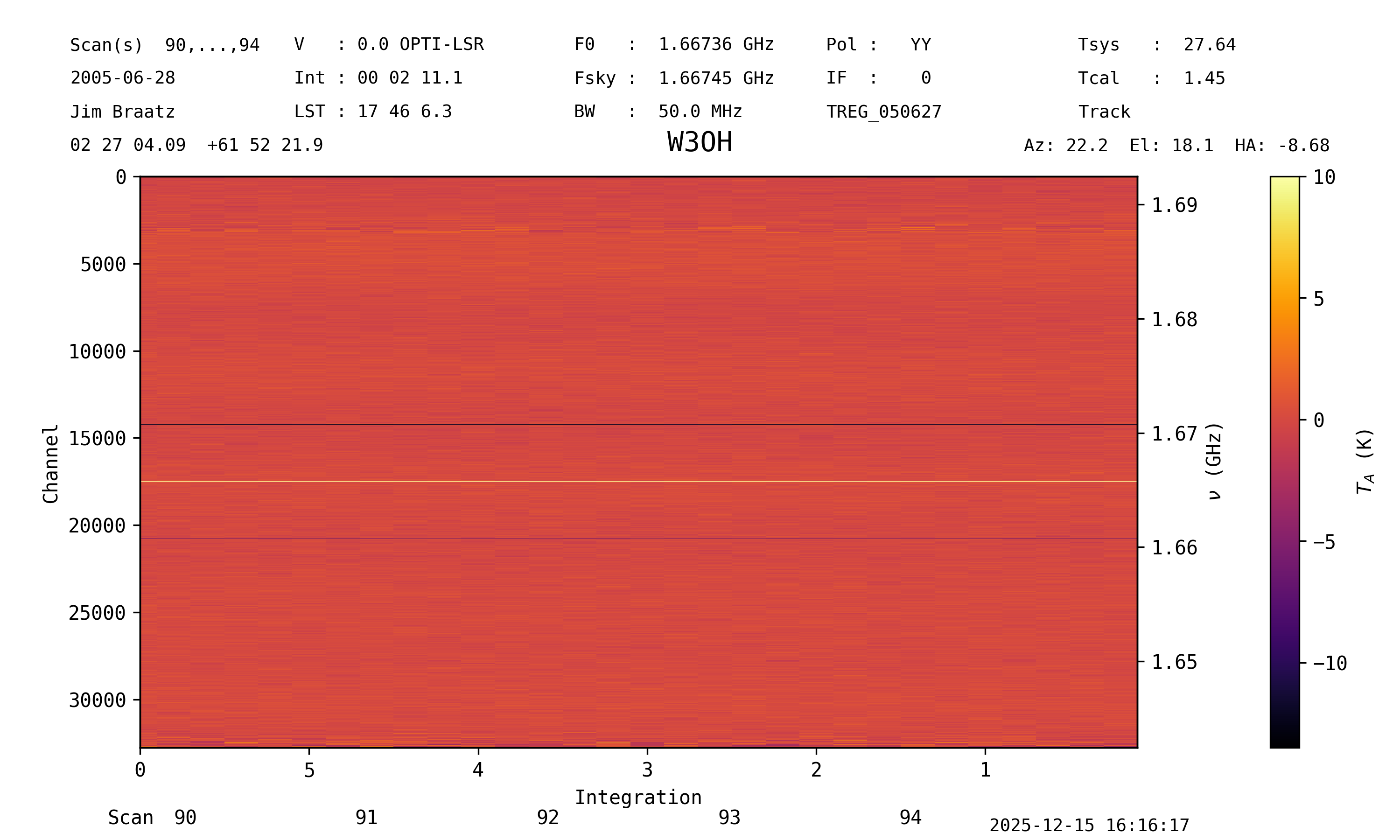
This method returns a ScanPlot object, which can be used to modify the plot.
See the waterfall plot guide for more details.
More details about the different calibration routines can be found on the calibration section of the users guide.
Time Averaging Data#
Time averaging the calibrated data into a single spectrum can be done using the ScanBlock.timeaverage method, like:
spectrum = scan_block.timeaverage()
This method returns a Spectrum object.
Plot the spectrum using the Spectrum.plot method:
spec_plot = spectrum.plot()
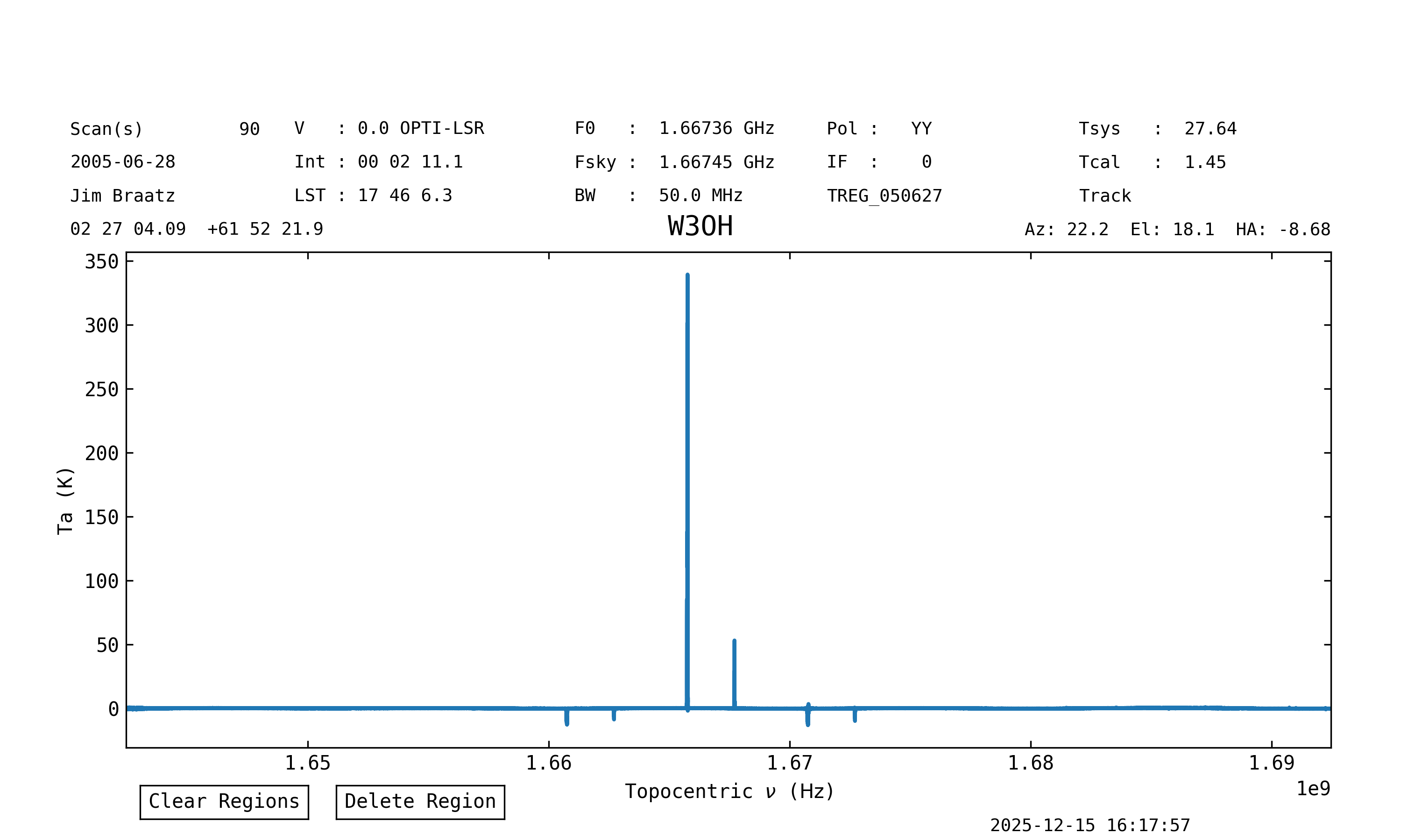
This method returns a SpectrumPlot object, which can be used to modify the plot.
See the spectrum plot guide for more details.
Baseline Removal#
To remove a baseline from the data use the Spectrum.baseline method.
This can use different polynomials to fit and remove a baseline from the spectrum.
To fit and remove a Chebyshev polynomial of degree 17, ignoring regions with spectral lines, and their ghosts, use:
# Define the channel ranges to be
# excluded from the baseline fit.
exclude = [(12720, 13259),
           (14060, 14440),
           (16000, 16420),
           (17375, 17640),
           (19355, 19660),
           (20575, 20955)]
spectrum.baseline(model="chebyshev", degree=17, remove=True, exclude=exclude)
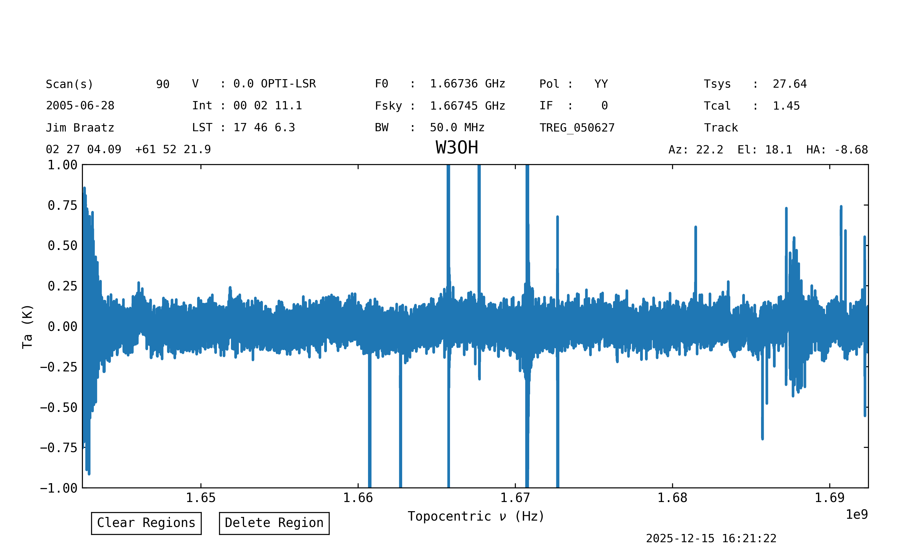
The spectrum has been baseline removed. The spectrum plot guide shows how to interactively include/exclude portions by clicking and dragging on the plot itself (without typing out all the tuples of 5-digit channel ranges)
Plot again, but focus on the line-free regions:
spec_plot = spectrum.plot(ymax=1, ymin=-1)
Polarization Average#
Polarization averaging can be done at the spectrum level, that is, after time averaging the data.
In this example we will calibrate the data for the second polarization (plnum=1) following the same steps as for the first one, and then average them together.
Calibrate, time average and baseline subtract the second polarization.
We use the same range of channels and baseline model to fit the baseline.
scan_block1 = sdfits.getfs(fdnum=0, ifnum=0, plnum=1)
spectrum1 = scan_block1.timeaverage()
spectrum1.baseline(model="chebyshev", degree=17, remove=True, exclude=exclude)
Now we proceed to average the spectra with the two polarizations, spectrum and spectrum1:
sp_avg = spectrum.average(spectrum1)
Slicing a Spectrum#
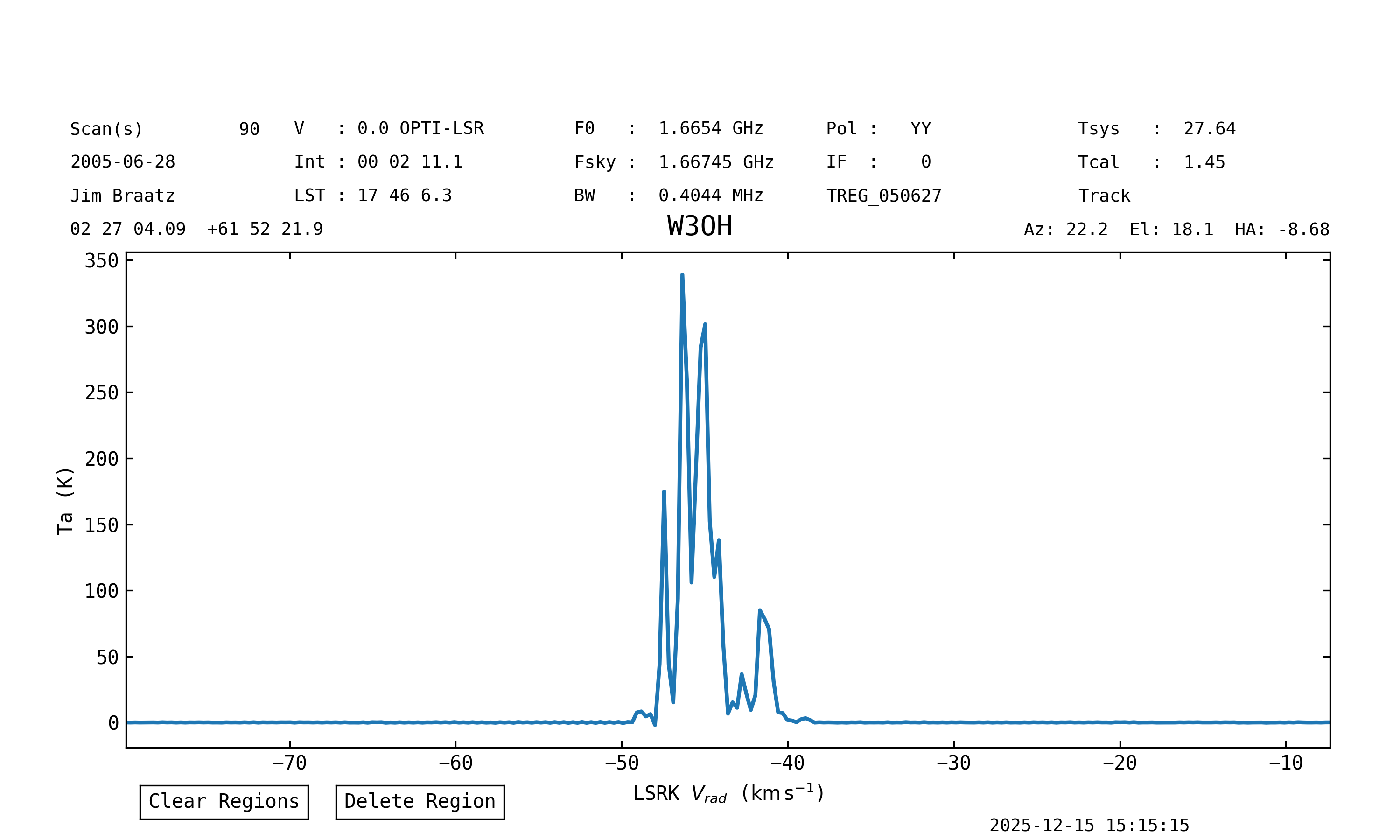
The brightest line is the OH maser at 1665.4018 MHz.
To crop the spectrum around this line we use a slice.
We will use astropy.units (imported automatically as u) to define the frequency range:
oh_bright_spec = spectrum[1665.3*u.GHz:1665.9*u.MHz]
Change the rest frequency to that of the 1665.4018 MHz line:
oh_bright_spec.doppler_rest = 1665.4018 * u.MHz
Plot in velocity units (xaxis_unit) using the local standard of rest as velocity frame (vel_frame) and the radio Doppler convention (doppler_convention):
oh_bright_spec.plot(xaxis_unit="km/s", vel_frame="lsrk", doppler_convention="radio")
Note that the setting the units, velocity frame or Doppler convention during plotting does not modify the spectrum.
Saving a Spectrum#
Save the spectrum to a FITS file (notice this is not SDFITS, for SDFITS use format=sdfits):
oh_bright_spec.write("W3OH_1665MHz_pol0.fits", format="fits")
Or to a text file:
oh_bright_spec.write("W3OH_1665MHz_pol0.txt", format="basic")
Reporting Issues#
If you find a bug or something you think is in error, please report it on the GitHub issue tracker. You must have a GitHub account to submit an issue.
Credits#
dysh is being developed by a partnership between the Green Bank Observatory and the Laboratory for Millimeter-wave Astronomy at the University of Maryland, College Park.