Nodding Data Reduction

Nodding Data Reduction#

This notebook shows the reduction path of a nodding observation with a multi-beam receiver, the K-band Focal Plane Array (KFPA).

Similar to a position-switched observation, two beams are selected for simultaneous observing (though the receiver can have more than two beams). In the first scan BEAM1 is looking at the source, while BEAM2 is looking at an assumed OFF position. In the next scan, BEAM2 will be looking at the source, while BEAM1 is looking at (another) OFF position. This will result in two position-switched solutions, which are then averaged for the final spectrum.

One advantage of this observing mode is that the telescope is always ON source, bringing the noise down by \(\sqrt{2}\) compared to a classic position switched observation. Minus a small amount of slewing time of course. However, the beam separation in the receiver should be large enough to ensure that the off position is not on the source. Otherwise, a proper Position Switching observation is needed with a large enough offset.

In the observations used in this tutorial there are also position switched observations of the same source, so we can compare the results of using beam nodding versus position switching.

The data in this tutorial were also presented in a similar GBTIDL data reduction.

Background#

The spectral line observed here is the NH\(_3\) (1,1) line at 23.69 GHz with the KFPA receiver. This receiver has 7 beams: one central beam and six beams in a roughly hexagonal pattern around the central beam. The source is a position in the W3 cloud, a roughly two degree sized Giant Molecular Cloud (GMC) with active star formation. See also https://herscheltelescope.org.uk/results/w3-star-forming-region/

Dysh commands#

The following dysh commands are introduced (leaving out all the function arguments):

  filename = dysh_data()
  sdf = GBTFITSLoad()
  sb = sdf.getnod()
  ta = sb.timeaverage()
  ta.baseline()
  ta.smooth()
  ta.average()
  ta.plot()
  ta.plot().spectrum

Loading Modules#

We start by loading the modules we will use for the data reduction.

# These modules are required for the data reduction.
from dysh.log import init_logging
from dysh.fits.gbtfitsload import GBTFITSLoad
from astropy import units as u

# These modules are used for file I/O
from dysh.util.files import dysh_data
from pathlib import Path

Setup Logging#

dysh uses a logger to communicate. If you are working in the command line, then the logging is setup for you. If you are working in a jupyter lab instance, then you need to set it up. You can do so using the init_logging function imported above. As an argument, init_logging takes a number, the verbosity level. level 0 is for error messages only, 1 for warning, 2 for info and 3 for debug. Here we set it to level 2.

init_logging(2)

# also create a local "output" directory where temporary notebook files can be stored.
output_dir = Path.cwd() / "output"
output_dir.mkdir(exist_ok=True)

Data Retrieval#

Download the example SDFITS data, if necessary.

filename = dysh_data(example="nod2")

00:11:47.558 I Resolving example=nod2 -> nod-KFPA/data/TGBT22A_503_02.raw.vegas.trim.fits

00:11:47.565 I url: http://www.gb.nrao.edu/dysh//example_data/nod-KFPA/data/TGBT22A_503_02.raw.vegas.trim.fits

Downloading TGBT22A_503_02.raw.vegas.trim.fits from http://www.gb.nrao.edu/dysh//example_data/nod-KFPA/data/TGBT22A_503_02.raw.vegas.trim.fits

00:11:47.837 I Starting download...

00:11:49.159 I Saved TGBT22A_503_02.raw.vegas.trim.fits to TGBT22A_503_02.raw.vegas.trim.fits

Retrieved TGBT22A_503_02.raw.vegas.trim.fits

Data Loading#

Next, we use GBTFITSLoad to load the data, and then its summary method to inspect its contents.

This trimmed dataset is an extraction from a much larger dataset (19GB) and can take some time to load if it’s the first time. This would be example="nod"

sdfits = GBTFITSLoad(filename)

sdfits.summary()

SCAN	OBJECT	VELOCITY	PROC	PROCSEQN	RESTFREQ	# IF	# POL	# INT	# FEED	AZIMUTH	ELEVATION
60	W3_1	-40.0	OnOff	1	23.694496	1	1	31	1	324.2279	38.7060
61	W3_1	-40.0	OnOff	2	23.694496	1	1	31	1	324.1526	39.0121
62	W3_1	-40.0	Nod	1	23.694496	1	1	31	7	324.2743	38.4194
63	W3_1	-40.0	Nod	2	23.694496	1	1	31	7	324.3672	38.2858

Data Reduction#

Nodding Data Reduction#

We start calibrating the Nod observations in scans 62 and 63. We use the GBTFITSLoad.getnod method to calibrate the data. This method will automatically find a pair of Nod scans given one scan number. It will also automatically figure out which feeds where used during the nodding observations. The return of getnod is a ScanBlock with at least two NodScan in it.

nodsb = sdfits.getnod(scan=62, ifnum=0, plnum=0)
nodsb

00:11:49.493 I Ignoring 1 blanked integration(s).

00:11:49.657 I Ignoring 1 blanked integration(s).

ScanBlock([NodScan scan=62 ifnum=0 (rest freq=23.69 GHz) plnum=0 (LL) fdnum=2 source='W3_1',
           NodScan scan=62 ifnum=0 (rest freq=23.69 GHz) plnum=0 (LL) fdnum=6 source='W3_1'])

Each NodScan holds all of the calibrated integrations for each feed used during the Nod observations. We can query the NodScan objects for information about the data, such as what is the system temperature, in K, or the exposure time, in seconds. NodScan is a sub class of a Scan object.

nodsb[0].tsys, nodsb[1].tsys

(array([64.0651583 , 65.84723928, 63.32246857, 64.9772735 , 63.77161495,
        62.82267302, 66.41525105, 62.88090753, 60.91140946, 62.18854417,
        60.81960096, 61.42624138, 59.32883166, 60.16711155, 61.45232073,
        60.71780304, 59.21079399, 62.45297224, 62.54435652, 64.53549963,
        65.65949202, 64.34252275, 64.24356553, 65.4308054 , 65.54581989,
        64.64741319, 62.45646939, 62.62895287, 61.91170188, 63.05362163]),
 array([73.42457338, 73.89318167, 77.95484204, 77.06676577, 79.64183646,
        80.67187842, 75.41180075, 74.18340271, 79.06335209, 82.58279698,
        78.22566126, 70.88384081, 68.7912057 , 69.28174137, 72.48114802,
        72.24762512, 74.46373175, 73.26477026, 73.02711593, 70.51565007,
        72.7222005 , 71.37948284, 71.11466717, 70.09686344, 70.74295942,
        69.47116087, 70.22771754, 67.13519555, 70.62961633, 69.03334933]))

nodsb[0].exposure, nodsb[1].exposure

(array([0.97587454, 0.97236673, 0.97587454, 0.97095654, 0.97587454,
        0.97587454, 0.97060335, 0.97587454, 0.97060334, 0.97587454,
        0.97587454, 0.97587454, 0.97060334, 0.97587454, 0.97060334,
        0.97587454, 0.97587454, 0.97095652, 0.97587454, 0.97095652,
        0.97587454, 0.97587454, 0.97060334, 0.97587454, 0.97060335,
        0.97587454, 0.97587454, 0.97060335, 0.97587454, 0.97587454]),
 array([0.97587454, 0.97201457, 0.97587454, 0.97095654, 0.97587454,
        0.97587454, 0.97095654, 0.97587454, 0.97060334, 0.97587454,
        0.97587454, 0.97587454, 0.97095654, 0.97587454, 0.97060334,
        0.97587454, 0.97587454, 0.97060334, 0.97587454, 0.97095652,
        0.97587454, 0.97587454, 0.97095654, 0.97587454, 0.97095654,
        0.97587454, 0.97587454, 0.97095654, 0.97587454, 0.97587454]))

nodsb[0].fdnum, nodsb[1].fdnum

(2, 6)

From the above we see that the beams used for nodding had fdnum of 2 and 6.

Inspecting Integrations#

To access the calibrated integrations we use the calibrated method of a Scan object. The return is a Spectrum object with the calibrated data. The argument to calibrated is the integration number.

nod_int = nodsb[0].getspec(0)
nod_int

<Spectrum(flux=[nan ... 1.7525686101720952] K (shape=(32768,), mean=3.35429 K); spectral_axis=<SpectralAxis 
   (observer: <ITRS Coordinate (obstime=2022-02-17T03:12:46.500, location=(0.0, 0.0, 0.0) km): (x, y, z) in m
                  (882593.9465029, -4924896.36541728, 3943748.74743984)
               (v_x, v_y, v_z) in km / s
                  (0., 0., 0.)>
    target: <SkyCoord (FK5: equinox=J2000.000): (ra, dec, distance) in (deg, deg, kpc)
                (36.37731467, 62.10479638, 1000000.)
             (pm_ra_cosdec, pm_dec, radial_velocity) in (mas / yr, mas / yr, km / s)
                (-3.65939096e-22, 0., -40.)>
    observer to target (computed from above):
      radial_velocity=-18.322117140068272 km / s
      redshift=-6.111413679055211e-05
    doppler_rest=23694495500.0 Hz
    doppler_convention=radio)
  [2.36845708e+10 2.36845715e+10 2.36845722e+10 ... 2.37080061e+10
 2.37080069e+10 2.37080076e+10] Hz> (length=32768))>

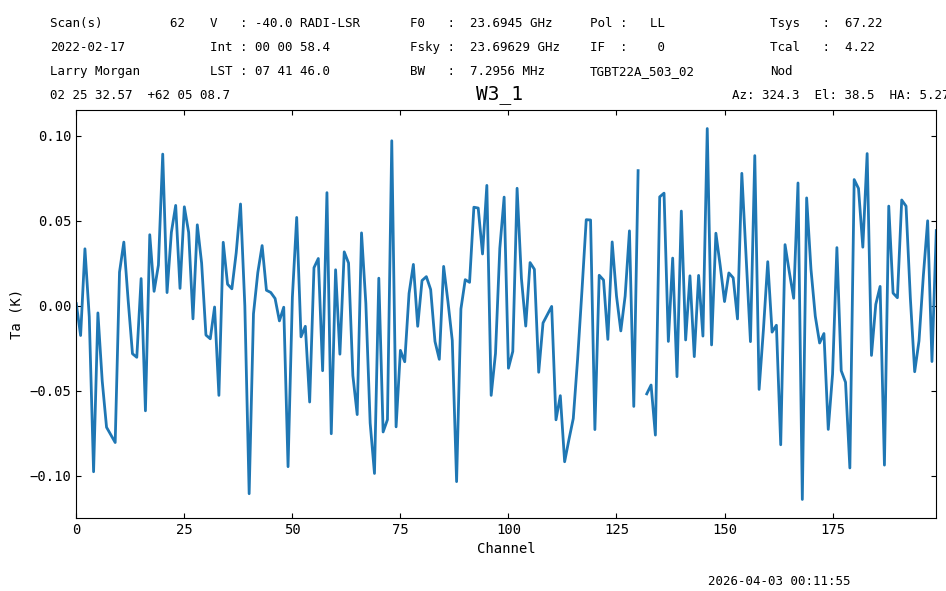
Spectrum objects have convenience functions to plot, smooth, and remove baselines, among others. Here we use the plot function to display the calibrated data for the first integration.

nod_int.plot()

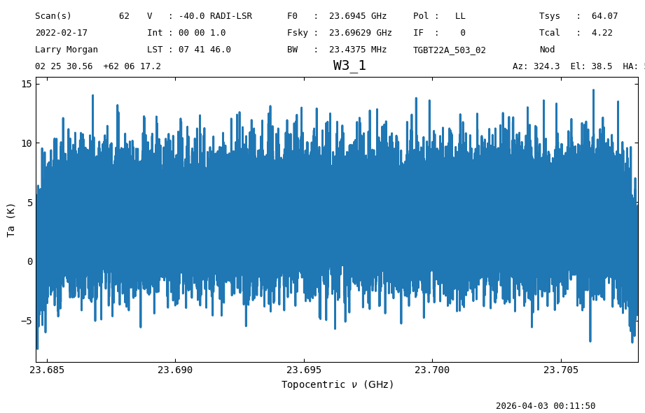
../_images/5646a95189e030acdc2237f85110addb46ba27844bf181b9568323eb560bffa9.png

<dysh.plot.specplot.SpectrumPlot at 0x71c671ed8790>

The plot shows a noise-like signal since it is only one 1 s integration. To see more details, and potentially a signal, we must time average the data.

Time Averaging#

To time average we can use the timeaverage function. We can use this function directly from a ScanBlock, in which case all of the data in the ScanBlock will be time averaged, or from a Scan, and only average the data inside the Scan. Here we will average all the data in the ScanBlock.

By default time averaging uses the following weights:

\[ \frac{T^{2}_{sys}}{\Delta\nu\Delta t} \]

with \(T_{sys}\) the system temperature, \(\Delta\nu\) the channel width and \(\Delta t\) the integration time. In dysh these are set using weights='tsys' (the default).

The return of timeaverage is a Spectrum object.

nod_ta = nodsb.timeaverage()
nod_ta

<Spectrum(flux=[-0.16442172102764782 ... -0.10698105320590709] K (shape=(32768,), mean=0.37476 K); spectral_axis=<SpectralAxis 
   (observer: <ITRS Coordinate (obstime=2022-02-17T03:12:46.500, location=(0.0, 0.0, 0.0) km): (x, y, z) in m
                  (882593.9465029, -4924896.36541728, 3943748.74743984)
               (v_x, v_y, v_z) in km / s
                  (0., 0., 0.)>
    target: <SkyCoord (FK5: equinox=J2000.000): (ra, dec, distance) in (deg, deg, kpc)
                (36.38569729, 62.08575673, 1000000.)
             (pm_ra_cosdec, pm_dec, radial_velocity) in (mas / yr, mas / yr, km / s)
                (-7.31878192e-22, 7.31878192e-22, -40.)>
    observer to target (computed from above):
      radial_velocity=-18.31506656233015 km / s
      redshift=-6.109062003167853e-05
    doppler_rest=23694495500.0 Hz
    doppler_convention=radio)
  [2.36845708e+10 2.36845715e+10 2.36845722e+10 ... 2.37080061e+10
 2.37080069e+10 2.37080076e+10] Hz> (length=32768))>

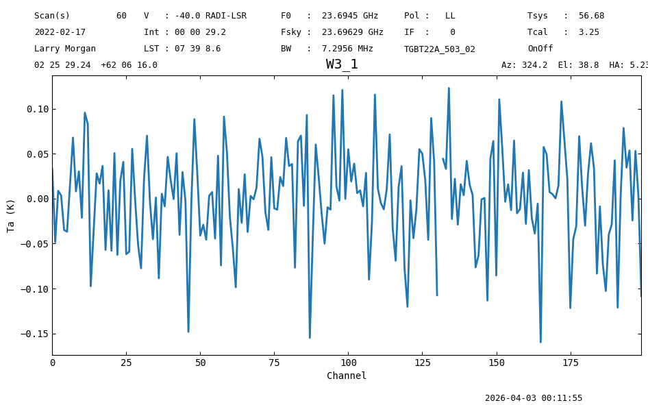
Now we plot the time average.

nod_ta.plot()

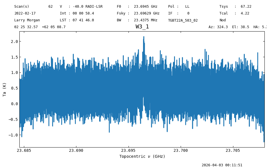
../_images/26290c30da2d64639ee578819e9737f5c691c2a86c91b4d9b80724dab4d902be.png

<dysh.plot.specplot.SpectrumPlot at 0x71c671ce7d90>

We see hints of a line. We can further reduce our data to bring out the signal from the noise.

Smoothing#

One way of reducing the noise in the time average is by smoothing the data along the spectral axis. This is done using the Spectrum.smooth function. The first argument is the kernel, and the second the width of the kernel in channels. The available kernels are a boxcar, Gaussian and a Hanning window. We use a boxcar with a width of 51 channels.

nod_ta_smooth = nod_ta.smooth('box', 51)

nod_ta_smooth.plot(xaxis_unit="GHz")

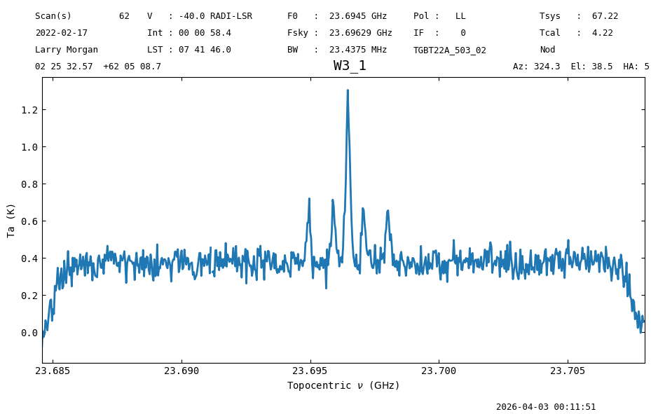
../_images/6870e74b7f0d34dd731ff2b3a8ea53c337db395484b8313b928803f87166685c.png

<dysh.plot.specplot.SpectrumPlot at 0x71c65fdfeef0>

The signal is clear now.

Statistics#

We can quantify the reduction in the noise using the Spectrum.stats function. To reduce the bias in the statistics, we will slice the spectrum to avoid the bandpass roll off channels. We use a channel range between 23.687 and 23.694 GHz.

s = slice(23.687*u.GHz, 23.694*u.GHz)

nod_ta_smooth[s].stats()  # rms 0.04587208 K

00:11:52.436 I Note: found 1 NaN (masked) values

{'mean': <Quantity 0.37603136 K>,
 'median': <Quantity 0.38060805 K>,
 'rms': <Quantity 0.04587208 K>,
 'min': <Quantity 0.26205572 K>,
 'max': <Quantity 0.48034968 K>,
 'npt': 191,
 'nan': np.int64(1)}

nod_ta[s].stats() # rms 0.33878936 K

00:11:52.805 I Note: found 52 NaN (masked) values

{'mean': <Quantity 0.3758673 K>,
 'median': <Quantity 0.36945952 K>,
 'rms': <Quantity 0.33836405 K>,
 'min': <Quantity -0.92130551 K>,
 'max': <Quantity 1.58757768 K>,
 'npt': 9787,
 'nan': np.int64(52)}

Before smoothing the rms was 339 mK, after smoothing it went down to 46 mK, so the reduction in the noise is 6% higher than \(\sqrt{51}\).

Baseline Subtraction#

Now we will subtract a baseline from the data. We use the Spectrum.baseline function to do it. We will ignore the edge channels and the region with line emission during the baseline fitting. This is specified with the exclude or include argument of baseline. Here we use include. Since the line free channels seem to have a flat frequency response, away from the window edges, we use an order 1 polynomial as our baseline model.

include = [(23.687*u.GHz, 23.694*u.GHz),
           (23.700*u.GHz, 23.705*u.GHz)
          ]
model = "poly"
order = 1

nod_ta_smooth.baseline(order, model=model, include=include, remove=True)

00:11:52.816 I EXCLUDING [Spectral Region, 1 sub-regions:
  (23684570787.125 Hz, 23687000000.0 Hz) 
, Spectral Region, 1 sub-regions:
  (23694000000.0 Hz, 23700000000.0 Hz) 
, Spectral Region, 1 sub-regions:
  (23705000000.0 Hz, 23707989690.47583 Hz) 
]

nod_ta_smooth.plot()

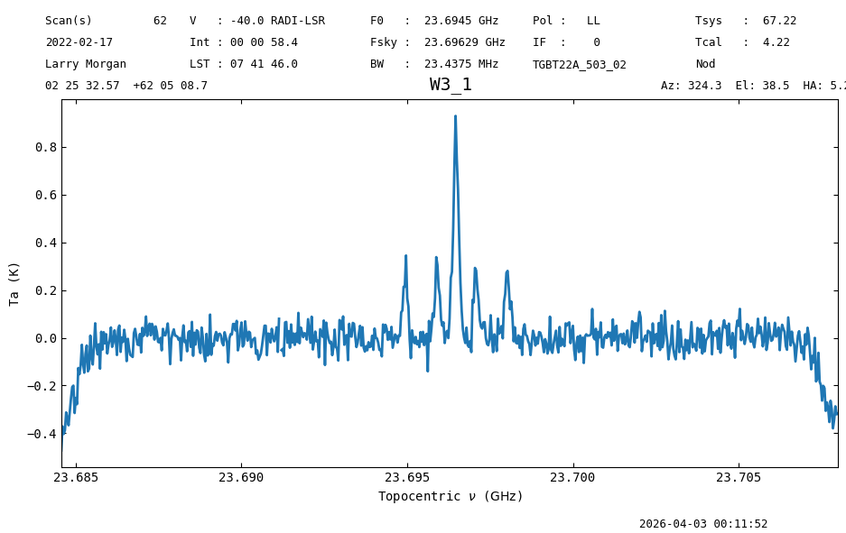
../_images/1891268d79eef92d4223b8e72c279aa609e4da2291d5410af90286ad5a891d5f.png

<dysh.plot.specplot.SpectrumPlot at 0x71c663f64d00>

Now we will proceed with the calibration of the OnOff observations for comparison.

OnOff Data Reduction#

Scans 60 and 61 contain OnOff observations (position switched). For the 7-beam KFPA receiver, the central beam (fdnum=0) will be the source tracking beam for the OnOff observations. As with the Nod calibration, dysh knows how to pair OnOff observations given a scan number. We use the GBTFITSLoad.getps function to calibrate position switched observations. As with getnod, the return of getps is a ScanBlock, but this time containing PSScan objects, which are also sub classes of the Scan class, so they share many of their functions and properties.

pssb = sdfits.getps(scan=60, plnum=0, ifnum=0, fdnum=0)
pssb

00:11:53.289 I Ignoring 1 blanked integration(s).

ScanBlock([PSScan scan=60 ifnum=0 (rest freq=23.69 GHz) plnum=0 (LL) fdnum=0 source='W3_1'])

We time average, smooth and baseline subtract the calibrated data. We use a chain of functions for the time averaging and smoothing.

ps_ta_smooth = pssb.timeaverage().smooth("box", 51)
ps_ta_smooth.baseline(order, model=model, include=include, remove=True)

00:11:53.563 I EXCLUDING [Spectral Region, 1 sub-regions:
  (23684570817.125 Hz, 23687000000.0 Hz) 
, Spectral Region, 1 sub-regions:
  (23694000000.0 Hz, 23700000000.0 Hz) 
, Spectral Region, 1 sub-regions:
  (23705000000.0 Hz, 23707989720.47583 Hz) 
]

ps_ta_smooth.plot(ymin=-0.2)

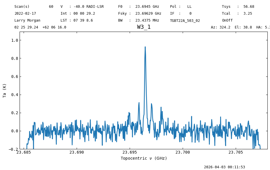
../_images/8bc58287c05da37e2ebb109ebd33b8ae86f1dc89fd50925b89d86e4419deab6a.png

<dysh.plot.specplot.SpectrumPlot at 0x71c663f645b0>

Comparing the Methods#

Both the Nod and OnOff scans shows a signal, How do the properties of the spectra compare?

# Line free rms
nod_ta_smooth[s].stats()["rms"], ps_ta_smooth[s].stats()["rms"]

00:11:54.153 I Note: found 1 NaN (masked) values

00:11:54.515 I Note: found 1 NaN (masked) values

(<Quantity 0.04586959 K>, <Quantity 0.0557227 K>)

The noise in the Nod spectrum is lower than that in the OnOff one. This makes sense since the exposure time in the Nod observations is almost twice as long as in the OnOff ones, for the same observing time. If that is the only factor, we would expect the noise in the Nod spectrum to be a factor \(\sqrt{2}\) lower than the OnOff one. Let’s check.

ps_ta_smooth[s].stats()["rms"]/nod_ta_smooth[s].stats()["rms"]/2**0.5

00:11:54.886 I Note: found 1 NaN (masked) values

00:11:55.248 I Note: found 1 NaN (masked) values

\[0.85899819 \; \mathrm{}\]

The ratio is 0.85, meaning that the noise reduction was 15% less than expected. This is likely because the system temperature of the feeds is different. Let’s check.

ps_ta_smooth.meta["TSYS"]/nod_ta_smooth.meta["TSYS"]

np.float64(0.8432606926356401)

The system temperature of the feed used for the OnOff observations is 15% lower than that of the feeds used for the Nod. This explains the observed difference in the noise.

The line peak is consistent between the Nod and OnOff spectra.

# Line peak
nod_ta_smooth.stats()["max"], ps_ta_smooth.stats()["max"]

00:11:55.262 I Note: found 1 NaN (masked) values

00:11:55.264 I Note: found 2 NaN (masked) values

(<Quantity 0.92860103 K>, <Quantity 0.9264315 K>)

# radiometer in a non-signal part of the spectrum:    (1.0043275608304512, 0.994918029194119) 
nod_ta_smooth[50:250].plot(xaxis_unit="chan").spectrum.radiometer(), ps_ta_smooth[50:250].plot(xaxis_unit="chan").spectrum.radiometer(),

../_images/67c710f1e36cbdfb21c75b46270522a7dd6881f6060cb1035fea212061e45fa8.png

00:11:55.477 I Note: found 1 NaN (masked) values

../_images/16a3b801b5f997ca5e8e0b21a262e59336dfd610b17a2b3e7621c5fa4d0d0281.png

00:11:55.685 I Note: found 1 NaN (masked) values

(np.float64(1.004327561874331), np.float64(0.9949180273182219))

Final Stats#

Finally, at the end we compute some statistics over a spectrum, merely as a checksum if the notebook is reproducible.

nod_ta_smooth.check_stats(0.11354235 * u.K)

00:11:55.693 I Note: found 1 NaN (masked) values

00:11:55.694 I rms is OK

Nodding Data Reduction

Contents

Nodding Data Reduction#

Background#

Dysh commands#

Loading Modules#

Setup Logging#

Data Retrieval#

Data Loading#

Data Reduction#

Nodding Data Reduction#

Inspecting Integrations#

Time Averaging#

Smoothing#

Statistics#

Baseline Subtraction#

OnOff Data Reduction#

Comparing the Methods#

Final Stats#