Flagging

This notebook shows how to use flags in dysh, as well as reminding on the concept of flagging vs. masking.

In dysh there are four sources of flags: a .flag file, user generated flags, flags generated from the SDFITS metadata (at present these only flag VEGAS channels known to be bad, i.e. VEGAS spurs), and the FLAGS column of the SDFITS binary table. The GBT does not produce data with a FLAGS column; however, dysh will write the FLAGS column if using GBTFITSLoad.write(flags=True) which is the default.

• Reading flags from a .flag file is controlled by the skipflags argument of GBTFITSLoad. By default this is set to False, as the default flags in a .flag file are VEGAS spurs, and those get flagged instead by looking at the SDFITS metadata. If you have generated flags in a .flag file, it must have the same name as the SDFITS file that it applies to but instead of ending in .fits it must end in .flag, and you must set skipflags=False when calling GBTFITSLoad. Lines in a flag file with IDSTRING VEGAS_SPUR are ignored by default, even if skipflags==True.

• Flags generated from the metadata are applied during the calibration process, e.g., when calling GBTFITSLoad.getsigref. For any of the calibration routines, the flagging of VEGAS spurs is controlled by the keyword flag_vegas. By default it is set to True, meaning that VEGAS spurs will be flagged. Once data is calibrated and VEGAS spur flags generated, these can be reverted in two ways. The first is to ignore all flags during calibration using apply_flags=False, the second is to clear all flags using GBTFITSLoad.clear_flags and repeat the calibration using flag_vegas=False.

• Flags in the FLAGS column are always read in if present and will be applied in a calibration method if apply_flags=True or if you call GBTFITSLoad.apply_flags. These flags can be cleared with GBTFITSLoad.clear_flags.

This notebook will explain how to generate your own flags using dysh, and show some examples of the two points above.

Dysh commands

The following dysh commands are introduced (leaving out all the function arguments):

  filename = dysh_data()
  sdf = GBTFITSLoad()
  sdf.flags.show()
  sdf.flags.clear()
  sdf.flag()
  sdf.clear_flags()
  sb = sdf.getps()
  sb.plot()
  sb.plot().write()

Loading Modules

We start by loading the modules we will use for this example.

# These modules are required for working with the data.
from dysh.fits.gbtfitsload import GBTFITSLoad
from dysh.util.selection import Selection
from dysh.log import init_logging
import numpy as np

# These modules are used for file I/O
from dysh.util.files import dysh_data
from pathlib import Path
import tarfile

# We also do some matplotlib here
import matplotlib.pyplot as plt

Setup

dysh uses a logger to communicate. If you are working in the command line, then the logging is setup for you. If you are working in a jupyter lab instance, then you need to set it up. You can do so using the init_logging function imported above. As an argument, init_logging takes a number, the verbosity level. level 0 is for error messages only, 1 for warning, 2 for info and 3 for debug. Here we set it to level

init_logging(2)

# also create a local "output" directory where temporary notebook files can be stored.
output_dir = Path.cwd() / "output"
output_dir.mkdir(exist_ok=True)

Data Retrieval

This time we download the data from a tar.gz file and then unpack it locally in the current “data” directory.

filename = dysh_data(example="rfi-L/data/AGBT17A_404_01.tar.gz")

00:10:02.350 I url: http://www.gb.nrao.edu/dysh//example_data/rfi-L/data/AGBT17A_404_01.tar.gz

Downloading AGBT17A_404_01.tar.gz from http://www.gb.nrao.edu/dysh//example_data/rfi-L/data/AGBT17A_404_01.tar.gz

00:10:02.620 I Starting download...

00:10:03.101 I Saved AGBT17A_404_01.tar.gz to AGBT17A_404_01.tar.gz

Retrieved AGBT17A_404_01.tar.gz

# Unpack.
with tarfile.open(filename) as targz:
    targz.extractall('./data/') 
    targz.close() 

Data Loading

After unpacking the data we load it. Notice how dysh tells us that it found an empty .flag file.

sdfits = GBTFITSLoad("./data/AGBT17A_404_01.raw.vegas", skipflags=False)

/home/docs/checkouts/readthedocs.org/user_builds/dysh/checkouts/release-1.1/src/dysh/util/selection.py:1377: UserWarning: Pandas doesn't allow columns to be created via a new attribute name - see https://pandas.pydata.org/pandas-docs/stable/indexing.html#attribute-access
  self._flag_file_rep = []
00:10:03.213 W No flag rules found in file data/AGBT17A_404_01.raw.vegas/AGBT17A_404_01.raw.vegas.A.flag

00:10:03.215 I Index loaded from .index file (44/93 columns). Missing columns (TCAL, WCS, calibration metadata, etc.) will be automatically loaded from FITS file when first accessed.

What flags were loaded?

sdfits.flags.show()

 ID TAG OBJECT BANDWID DATE-OBS ... SUBOBSMODE FITSINDEX CHAN UTC # SELECTED
--- --- ------ ------- -------- ... ---------- --------- ---- --- ----------

The above shows that the .flag file was empty, so no flags were loaded.

Now, lets look at the summary.

sdfits.summary()

SCAN	OBJECT	VELOCITY	PROC	PROCSEQN	RESTFREQ	# IF	# POL	# INT	# FEED	AZIMUTH	ELEVATION
19	A123606	6600.0	OnOff	1	1.420406	1	2	61	1	64.5805	48.3795
20	A123606	6600.0	OnOff	2	1.420406	1	2	61	1	64.6012	48.4338

Data Inspection

There are two scans, a pair of position switched observations. We will calibrate it and see how the data looks like.

We start by looking at the time average of the calibrated data.

# Calibrate the data.
ps_scanblock = sdfits.getps(scan=19, plnum=0, ifnum=0, fdnum=0)

# Compute the time average.
ps = ps_scanblock.timeaverage()

# Plot.
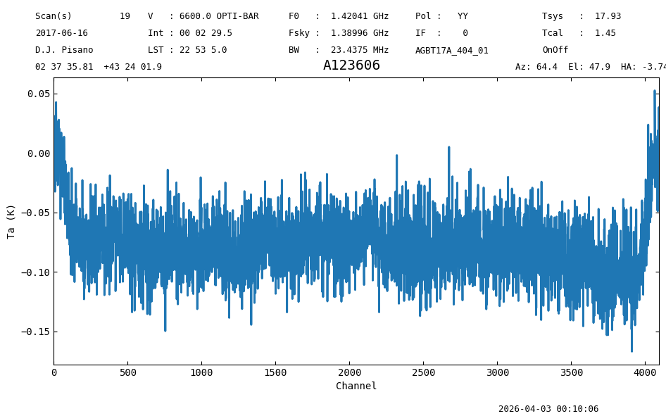
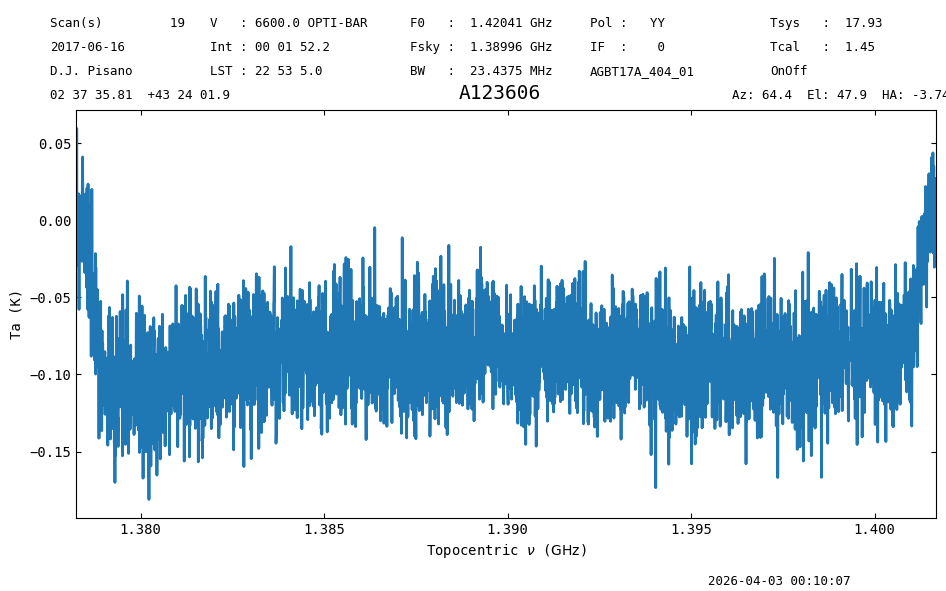
ps.plot(xaxis_unit="chan");

00:10:03.469 I Ignoring 1 blanked integration(s).

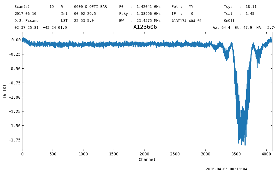
There is radio frequency interference (RFI) for channels above ~2300. We will plot a waterfall to see if the RFI is confined in time. This is done using the plot method of a ScanBlock.

psp = ps_scanblock.plot()

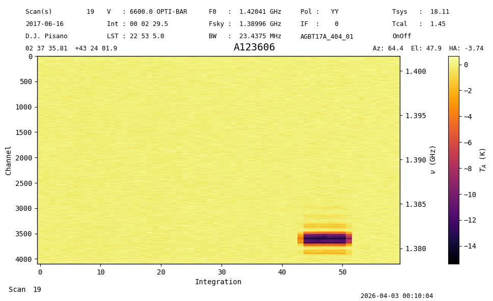
The RFI is confined to integrations 42 to 52, and it affects channels >2300. We will flag this range. Since the RFI shows as negative, it is also likely that this is present in the off scan, scan=20. The central frequency of the RFI is 1.381 GHz, which is a notorious GPS signal that shows up intermittendly.

tp_scanblock = sdfits.gettp(scan=[19,20], plnum=0, ifnum=0, fdnum=0)
tp_scanblock.plot();

00:10:05.323 I Ignoring 1 blanked integration(s).

00:10:05.425 I Ignoring 1 blanked integration(s).

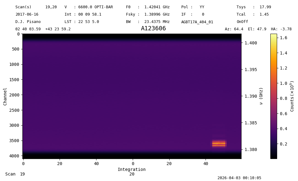
So it turns out the RFI is only in the OFF, explaining the negative signal. Although it is possible to flag just those integrations, and get slightly better S/N, we leave this as an excerize for the reader.

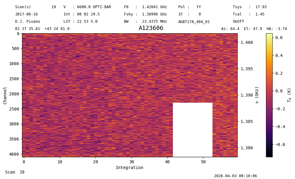
Although the current plot gives a good overview, another more interactive view can be done using a FITS file. You will need to emply common 3rd party tools such as ds9 , QFitsView or carta . Here is an example how to create a subsection of the figure above.

psp.write(output_dir / 'A123606_waterfall.fits', avechan=4, chan=[3000,4000], overwrite=True)

00:10:06.120 I Wrote /home/docs/checkouts/readthedocs.org/user_builds/dysh/checkouts/release-1.1/docs/source/users_guide/output/A123606_waterfall.fits with size 60 x 250

Data Flagging

We use the GBTFITSLoad.flag method to generate flags.

sdfits.flags.clear()
sdfits.flag(scan=20, 
            channel=[[2300,4096]], 
            intnum=[i for i in range(42,53)])
sdfits.flags.show()

 ID    TAG    SCAN             INTNUM                 CHAN     # SELECTED
--- --------- ---- ----------------------------- ------------- ----------
  0 d1edcbee4   20 [42,43,44,45,...,49,50,51,52] [[2300,4096]]         44

Careful readers might notice there is no channel 4096, since channels are numbered 0 to 4095 here. However, in this context of flagging it does no harm.

We repeat the calibration after generating the flags.

pssb = sdfits.getps(scan=19, plnum=0, fdnum=0, ifnum=0, apply_flags=True)

pssb.plot();

00:10:06.259 I Ignoring 1 blanked integration(s).

The channels and times affected by RFI have been flagged. We can time average to generate the final spectrum without the RFI.

ps = pssb.timeaverage()
ps.plot(xaxis_unit="chan");

Removing Flags

To remove flags from the GBTFITSLoad object use the clear_flags method.

sdfits.clear_flags()
sdfits.flags.show()

 ID TAG OBJECT BANDWID DATE-OBS ... SUBOBSMODE FITSINDEX CHAN UTC # SELECTED
--- --- ------ ------- -------- ... ---------- --------- ---- --- ----------

Statistics-based Flagging

We can assume that any significant increase in the standard deviation of the raw spectra is due to heavy RFI. Below, we will calculate \(\mu + 3\sigma\) for each of the 8 individual switching states, and flag any integrations breaching that threshold. Here \(\mu\) is the mean, and \(\sigma\) the standard deviation.

The last integration has been blanked by VEGAS, and is not plotted below.

#Get raw spectra and standard deviations
specs = sdfits.rawspectra(0,0)
stdevs = np.std(specs,axis=1)


#Organize into scan and switching state.
#There are 2 scans for the target and reference pointings, 2 calibration diode states, and 2 polarizations.
stdevs = np.reshape(stdevs, (2,-1,4))

nrows = stdevs.shape[1]

#Inspect the data  (last integration is removed, it has issues)
for scan in range(2):
    for sw_state in range(4):
        plt.plot(stdevs[scan,:-1,sw_state],label=f'State {(4*scan)+sw_state}')
        
plt.xlabel('Integration #')
plt.ylabel('sigma')
plt.legend()
plt.show()

/home/docs/checkouts/readthedocs.org/user_builds/dysh/envs/release-1.1/lib/python3.10/site-packages/traitlets/traitlets.py:1385: DeprecationWarning: Passing unrecognized arguments to super(Toolbar).__init__().
NavigationToolbar2WebAgg.__init__() missing 1 required positional argument: 'canvas'
This is deprecated in traitlets 4.2.This error will be raised in a future release of traitlets.
  warn(

We can see that the 4 states corresponding to the OFF scan have a significant jump corresponding to the GPS L3 RFI. It does not appear to start until the 40th integration, so we will use that as our cutoff to calculate the statistics of the good data, and the thresholds to flag by.

flag_mask = np.zeros(stdevs.shape)
cutoff = 40

mean = np.nanmean(stdevs[:,:cutoff,:],axis=1)
spread = 3 * np.nanstd(stdevs[:,:cutoff,:],axis=1)

Now we create our flagging mask of zeros and ones, where a one corresponds to a flag to be applied.

flag_mask = np.zeros(stdevs.shape)

mean = np.expand_dims(mean,axis=1)
spread = np.expand_dims(spread,axis=1)

flag_mask[stdevs > mean+spread] = 1
flag_mask = flag_mask.flatten()

flag_rows = np.where(flag_mask==1)[0].tolist()
print(flag_rows)

[176, 178, 185, 186, 187, 190, 191, 194, 195, 198, 199, 201, 202, 203, 206, 207, 208, 209, 210, 211, 214, 215, 216, 217, 218, 219, 222, 223, 226, 227, 230, 231, 234, 235, 236, 237, 238, 239, 240, 242, 416, 417, 418, 419, 420, 421, 422, 423, 424, 425, 426, 427, 428, 429, 430, 431, 432, 433, 434, 435, 436, 437, 438, 439, 440, 441, 442, 443, 444, 445, 446, 447, 448, 449, 450, 451, 484, 486]

We apply the flags using the “row” keyword, and see that the RFI is removed, along with a drop in the exposure time to 112 seconds instead of the original 150.

sdfits.flag(row=flag_rows)


ps = sdfits.getps(plnum=0, ifnum=0, fdnum=0).timeaverage()
print(f"Exposure: {ps.meta['EXPOSURE']} s")

ps.plot();

Exposure: 112.15101951854204 s

Flags vs. Masks

A few words on flagging vs. masking. Flagging sets the rule. apply_flags or calibrating with apply_flags=True (the default) sets the data mask. By default GBTFITSLoad will not read flag files. The keywords skipflags= and flag_vegas= control which flags are applied. flag_vegas can also be given as a parameter to any calibration routine, as below with gettp.

For a given spectrum the stats function reports the number of “nan”, which should be the number of channels that were masked as a result of flagging.

Note: If you change the Spectrum.mask attribute, it will be reflected in the plot, but not in the flags of the Spectrum if you write it out. Such a mask change should be considered temporary; to correctly change both the mask and the flag, use a flagging operation.

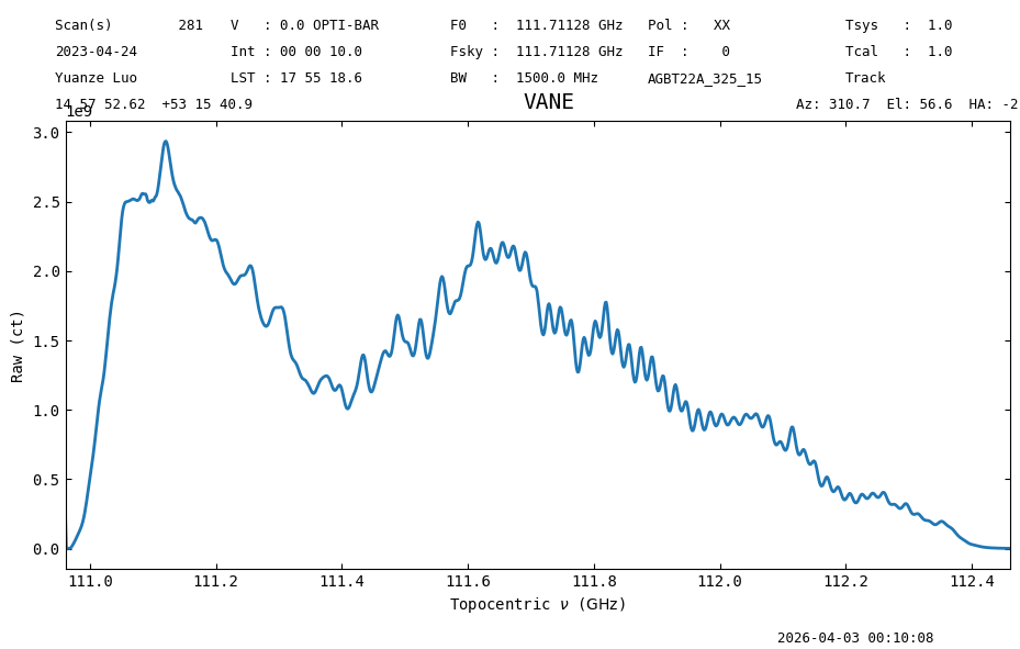
sdf1 = GBTFITSLoad(dysh_data(test="AGBT22A_325_15"))
sp1 = sdf1.gettp(scan=281, ifnum=0, plnum=0, fdnum=8, flag_vegas=True).timeaverage()
sp1.plot();

00:10:07.975 I Loaded 2 FITS files

00:10:07.976 I Index loaded from .index file (44/93 columns). Missing columns (TCAL, WCS, calibration metadata, etc.) will be automatically loaded from FITS file when first accessed.

00:10:08.125 I Using TSYS column

Looking carefully in this plot, you will see numerous “gaps” in the spectrum, where the so-called VEGAS spurs were automatically flagged. Using the stats function you will see there are 31 in this spectrum of 1024 channels. These are “nan” values in the spectrum, and the sp1.mask array has been set appropriately.

In the corresponding AGBT22A_325_15.raw.vegas.A.flag file you will see the following:

[header]
created = Tue Aug 20 09:38:32 2024
version = 1.0
created_by = sdfits
[flags]
#RECNUM,SCAN,INTNUM,PLNUM,IFNUM,FDNUM,BCHAN,ECHAN,IDSTRING
*|281|*|*|0|8|0,32,64,96,128,160,192,224,256,288,320,352,384,416,448,480,544,576,608,640,672,704,736,768,800,832,864,896,928,960,992|0,32,64,96,128,160,192,224,256,288,320,352,384,416,448,480,544,576,608,640,672,704,736,768,800,832,864,896,928,960,992|VEGAS_SPUR
*|281|*|*|0|10|0,32,64,96,128,160,192,224,256,288,320,352,384,416,448,480,544,576,608,640,672,704,736,768,800,832,864,896,928,960,992|0,32,64,96,128,160,192,224,256,288,320,352,384,416,448,480,544,576,608,640,672,704,736,768,800,832,864,896,928,960,992|VEGAS_SPUR

sp1.stats()

{'mean': <Quantity 1.25568126e+09 ct>,
 'median': <Quantity 1.26138573e+09 ct>,
 'rms': <Quantity 7.4497802e+08 ct>,
 'min': <Quantity 849293.34375 ct>,
 'max': <Quantity 2.9360649e+09 ct>,
 'npt': 1024,
 'nan': np.int64(31)}

Repeating this while ignoring all the flags (apply_flags=False) will show a contiguous spectrum and no masked channels.

sp2 = sdf1.gettp(scan=281, ifnum=0, plnum=0, fdnum=8, apply_flags=False).timeaverage()
sp2.plot()
sp2.stats()

00:10:08.511 I Using TSYS column

{'mean': <Quantity 1.25571771e+09 ct>,
 'median': <Quantity 1.2609328e+09 ct>,
 'rms': <Quantity 7.44805174e+08 ct>,
 'min': <Quantity 849293.34375 ct>,
 'max': <Quantity 2.9360649e+09 ct>,
 'npt': 1024,
 'nan': np.int64(0)}

Final Stats

Finally, at the end we compute some statistics over a spectrum, merely as a checksum if the notebook is reproducible.

ps.check_stats(0.02860246)

00:10:08.839 I rms is OK  (no unit was given, assumed K)