Position-Switched Data Reduction

Position-Switched Data Reduction#

This notebook shows how to use dysh to calibrate an OnOff observation. It retrieves and calibrates position-switch scans using GBTFITSLoad.getps, which returns a ScanBlock object. These in turn can be averaged into a Spectrum. OffOn observations can be reduced the same way.

Dysh commands#

The following dysh commands are introduced (leaving out all the function arguments):

  filename = dysh_data()
  sdf = GBTFITSLoad()
  sdf.select()
  sb = sdf.getps()
  ta = sb.timeaverage()
  ta.baseline()
  ta.average()
  ta.plot()
  ta_plt.savefig()

Loading Modules#

We start by loading the modules we will use for the data reduction.

# These modules are required for the data reduction.
from dysh.fits.gbtfitsload import GBTFITSLoad
from astropy import units as u
from dysh.log import init_logging

# These modules are used for file I/O
from dysh.util.files import dysh_data
from pathlib import Path

Setup#

dysh uses a logger to communicate. If you are working in the command line, then the logging is setup for you. If you are working in a jupyter lab instance, then you need to set it up. You can do so using the init_logging function imported above. As an argument, init_logging takes a number, the verbosity level. level 0 is for error messages only, 1 for warning, 2 for info and 3 for debug. Here we set it to level 2.

init_logging(2)

# also create a local "output" directory where temporary notebook files can be stored.
output_dir = Path.cwd() / "output"
output_dir.mkdir(exist_ok=True)

Data Retrieval#

Download the example SDFITS data, if necessary. The actual filename will depend on your dysh installation, it could be local, or it will need to be downloaded.

The dysh_data function has a few mnemonics, to avoid having to remember long filenames.

filename = dysh_data(test="getps")

00:12:39.943 I Resolving test=getps -> AGBT05B_047_01/AGBT05B_047_01.raw.acs/

Data Loading#

Next, we use GBTFITSLoad to load the data, and then its summary method to inspect its contents.

sdfits = GBTFITSLoad(filename)

00:12:39.997 I Index loaded from .index file (44/93 columns). Missing columns (TCAL, WCS, calibration metadata, etc.) will be automatically loaded from FITS file when first accessed.

sdfits.summary()

SCAN	OBJECT	VELOCITY	PROC	PROCSEQN	RESTFREQ	# IF	# POL	# INT	# FEED	AZIMUTH	ELEVATION
51	NGC5291	4386.0	OnOff	1	1.420405	1	2	11	1	198.3431	18.6427
52	NGC5291	4386.0	OnOff	2	1.420405	1	2	11	1	198.9306	18.7872
53	NGC5291	4386.0	OnOff	1	1.420405	1	2	11	1	199.3305	18.3561
54	NGC5291	4386.0	OnOff	2	1.420405	1	2	11	1	199.9157	18.4927
55	NGC5291	4386.0	OnOff	1	1.420405	1	2	11	1	200.3042	18.0575
56	NGC5291	4386.0	OnOff	2	1.420405	1	2	11	1	200.8906	18.1860
57	NGC5291	4386.0	OnOff	1	1.420405	1	2	11	1	202.3275	17.3853
58	NGC5291	4386.0	OnOff	2	1.420405	1	2	11	1	202.9192	17.4949

Here the PROCSEQN designates which scan is the “On” (1) and which the Off (2). If you like to see more columns, use the add_columns argument to summary, as we saw in the managing metadata notebook.

Data Reduction#

Single Scan#

Next we calibrate one scan of the position switched observations. We will start with scan 51, a single spectral window, polarization and feed.

ps_scan_block = sdfits.getps(scan=51, ifnum=0, plnum=0, fdnum=0)

print(f"T_sys = {ps_scan_block[0].tsys.mean():.2f}")

T_sys = 19.36

Time Averaging#

To time average the contents of a ScanBlock use its timeaverage method. Be aware that time averging will not check if the source is the same.

By default time averaging uses the following weights:

\[ \frac{T^{2}_{sys}}{\Delta\nu\Delta t} \]

with \(T_{sys}\) the system temperature, \(\Delta\nu\) the channel width and \(\Delta t\) the integration time. In dysh these are set using weights="tsys" (the default).

ta = ps_scan_block.timeaverage(weights="tsys")

Plotting#

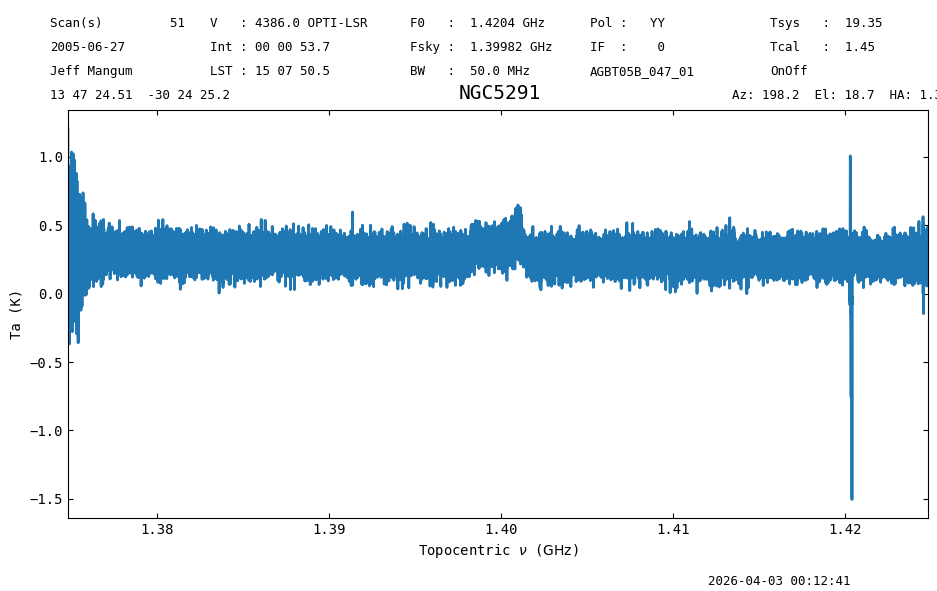
Plot the data and use different units for the spectral axis. Without any arguments it will auto-scale.

ta.plot();

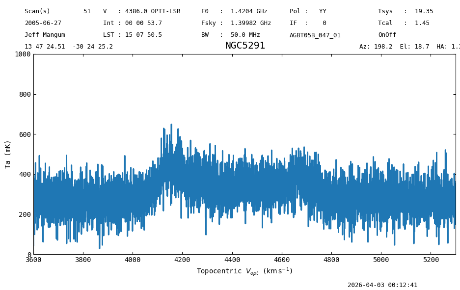
../_images/c592b4bc04d43ba17a509654347ad711d8d33683997c6c77327df1403a2bceba.png

Change the spectral axis units to km/s and the y-axis to mK, while also showing the spectra between 3600 and 5300 km/s, with the y-axis range between 0 and 1000 mK. Notice a small amount of “continuum” is left, most likely due to the varying sky in this OnOff positionswitch observation. We will need to perform a baseline subtraction later on in this notebook.

ta.plot(xaxis_unit="km/s", yaxis_unit="mK", ymin=0, ymax=1000, xmin=3600, xmax=5300);

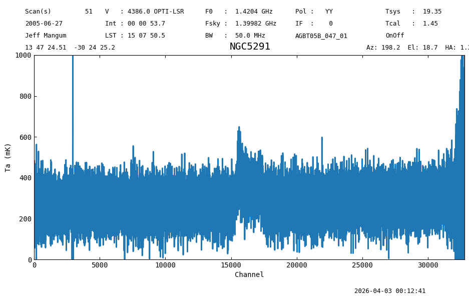
../_images/4b0d0ddfbfb41423ef7c5f1edb51678772e193db50079e02fe718af04fc08b91.png

Switch to channels as the spectral axis unit.

Notice we are also returning a plotter object (plt1) so we can save it later with as baseline fit.

plt1 = ta.plot(xaxis_unit="chan", ymin=0, ymax=1000, yaxis_unit="mK")

../_images/53a52c4fdc67365e9f79eea8c1d08dc314f8c201616051249d356887ab8f29e3.png

Baseline Subtraction#

The following code cells show how to subtract a polynomial baseline from the data. This example uses an 2nd order polynomial, and excludes the regions between 3800 and 5000 km/s, where a line is detected. The use of remove=True will remove the best fit baseline model from the spectrum, but by default the baseline is not subtracted. This will show that plotting the spectrum will also display the fitted baseline. (caveat: only the last plot before the baseline fit).

For a polynomial model one may need to normalize the frequency axis in channel space using normalize=True, to prevent poorly conditioned fits, but this will not allow you to undo the fit.

kms = u.km/u.s
ta.baseline(model="poly", degree=2, exclude=[3800*kms,5000*kms]) 
#  saving the plot will also show the baseline fit
plt1.savefig(output_dir / "plt1.png")

00:12:42.025 I EXCLUDING [Spectral Region, 1 sub-regions:
  (1397103816.4779327 Hz, 1402626103.134255 Hz) 
]

Notice that in interactive mode you would see the fitted baseline in the spectrum plot before. But in normal notebook mode, the figure needs to be saved explicitly. Re-executing the cell will overplot new baseline fits.

Now remove the baseline for sure. Again, this is not the default.

ta.baseline(model="poly", degree=2, exclude=[3800*kms,5000*kms], remove=True)

00:12:42.390 I EXCLUDING [Spectral Region, 1 sub-regions:
  (1397103816.4779327 Hz, 1402626103.134255 Hz) 
]

As an aside, exluding the obvious signal for NGC5291, will however include the edges, and the galactic emission around 0 km/s. It would be better to use the include= keyword and give a list of two intervals, for example 500 to 3800 and 5000 to 9000 km/s. We leave this as an exersize for the reader. You should find a difference of about 7 mK between the two solutions.

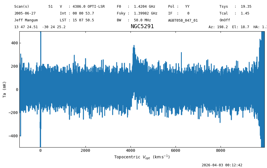
When we plot the spectrum again, it has been baseline subtracted.

plt2 = ta.plot(xaxis_unit="km/s", yaxis_unit="mK", ymin=-500, ymax=500)

../_images/af08abd11289249d27acc734270f0e3e1c750faac06a65c5f377ed36712c5e66.png

We can inspect the best fit baseline coefficients.

print(ta.baseline_model)

<QuantityModel Polynomial1D(2, c0=0.27098987, c1=0.02448574, c2=0.01186811, domain=(np.float64(1424816838.1210938), np.float64(1374818364.0))), input_units=Hz, return_units=K>

And save the figure, now without a baseline fit of course.

plt2.savefig(output_dir / "baselined_removed.png")

If for some reason you are not happy, use the ta.undo_baseline() function to restore the Spectrum data and delete the baseline model. You can then start with a new baseline fit.

Using Selection#

The following code shows how to calibrate scan 51 using selection. Selection does not know about signal and reference scan pairs, so the selection must include both scans, otherwise the calibration will fail.

sdfits.select(scan=[51,52])
sdfits.selection.show()

 ID    TAG      SCAN  # SELECTED
--- --------- ------- ----------
  0 0aa77fac2 [51,52]         88

sb = sdfits.getps(plnum=0, ifnum=0, fdnum=0)

ta2 = sb.timeaverage(weights='tsys')
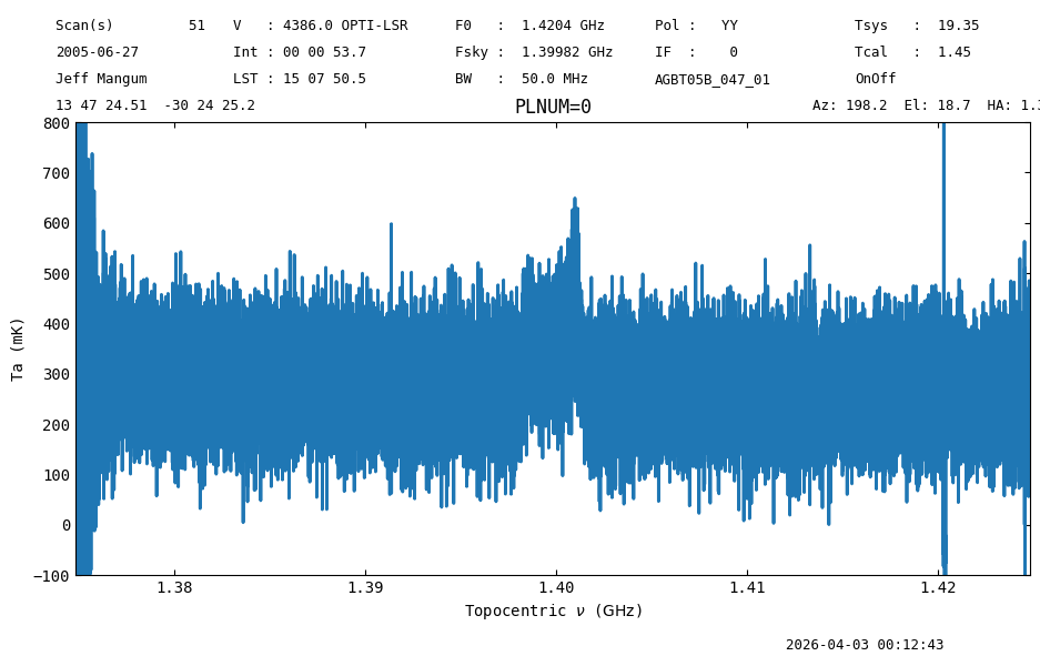
ta2.plot(xaxis_unit="GHz", ymin=-100, ymax=800, yaxis_unit="mK", title="PLNUM=0");

../_images/f4f8c8054d534ae5ceaff6a5218ab5ded8a89b6e54c3f215e79d376ecc5d21b7.png

We can calibrate the other polarization, with the scan numbers already selected.

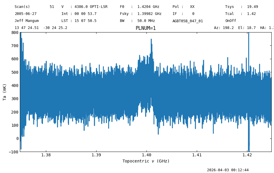
sb = sdfits.getps(plnum=1, fdnum=0, ifnum=0)
ta3 = sb.timeaverage(weights='tsys')
ta3.plot(xaxis_unit="GHz", ymin=-100, ymax=800, yaxis_unit="mK", title="PLNUM=1");

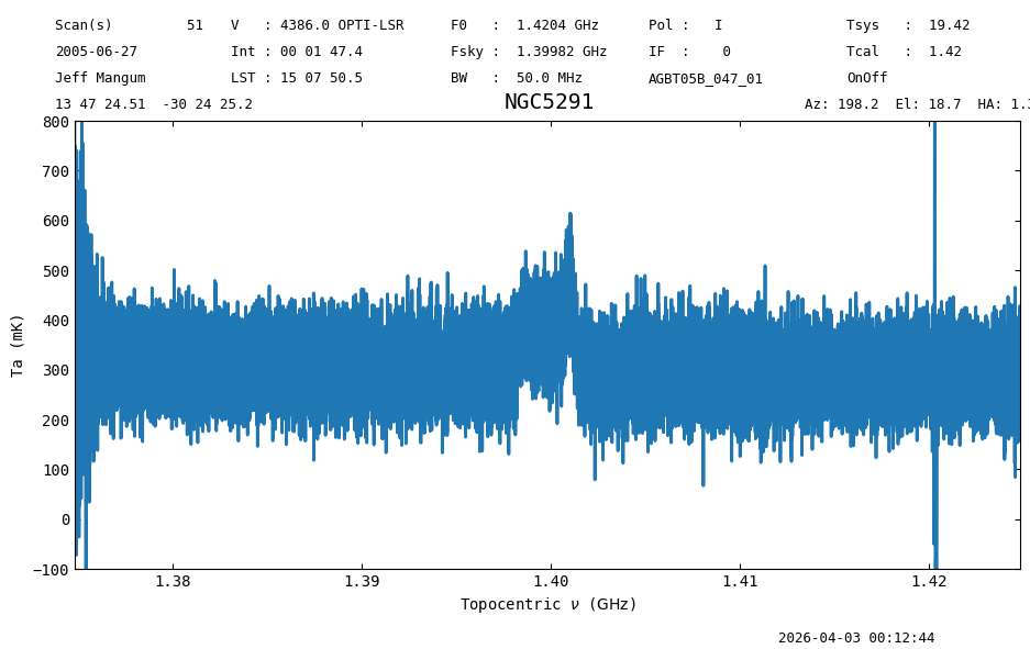
../_images/7d560db5b2a42134d15eea76195b21269aed9ccc9d27c1c0e39dd5c09608503d.png

Polarization Average#

Average the polarizations and plot the result.

avg = ta2.average(ta3)
avg.plot(ymin=-100, ymax=800, yaxis_unit="mK", xaxis_unit="GHz");

../_images/a1b6345d44339b4e1901e188b9a713e2a4af03c2477cb968837234bfdf642b31.png

All Scans#

Now we leverage the power of dysh to calibrate and time average all of the scans in the data.

We start by clearing the selection, so all of the scans are available.

sdfits.clear_selection()

Then, make a ScanBlock for spectral window 0, polarization 0, and feed 0. Time average the scans in the ScanBlock into a single Spectrum and then remove a baseline.

ps_scan_block_0 = sdfits.getps(ifnum=0, plnum=0, fdnum=0)
ps_ta_0 = ps_scan_block_0.timeaverage(weights='tsys')
ps_ta_0.baseline(model="poly", degree=2, exclude=[3800*kms,5000*kms], remove=True)

00:12:46.054 I EXCLUDING [Spectral Region, 1 sub-regions:
  (1397103816.4779327 Hz, 1402626103.134255 Hz) 
]

Now plot and compare with the result for a single scan.

ta.plot(ymin=-400, ymax=400, yaxis_unit="mK", xaxis_unit="GHz")
ps_ta_0.plot(ymin=-400, ymax=400, yaxis_unit="mK", xaxis_unit="GHz");

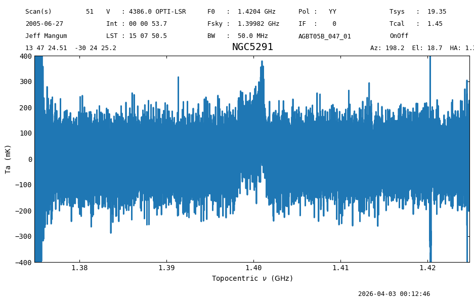
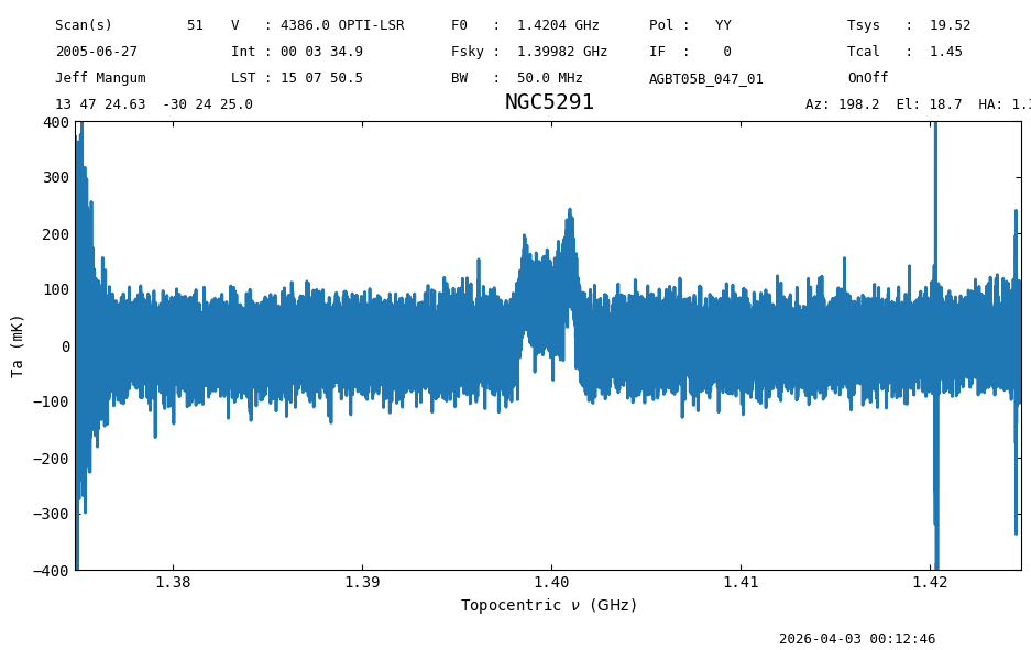
../_images/bf5cf4ec9bee122f3773326923391461b0149b04a75cf29a02e2f7a8838d0aac.png

../_images/10a3e5c884f890ae18508ef3d5e9ece26ddf80090b5a08507d9a7adc8768513c.png

The rms in the second Figure is almost half that of the first Figure. That is because there are four pairs of position switched scans in the data, so that results in a factor of \(\sqrt{4}\) reduced noise when we average all the data.

Final Stats#

Finally, at the end we compute some statistics over a spectrum, merely as a checksum if the notebook is reproducible.

ps_ta_0.check_stats(0.06010087 * u.K)

00:12:46.829 I rms is OK