SubBeamNod Data Reduction#
This notebook shows how to use dysh to calibrate an SubBeamNod observation via two different methods. It retrieves and calibrates SubBeamNod scans using GBTFITSLoad.subbeamnod() which returns a ScanBlock object.
Dysh commands#
The following dysh commands are introduced (leaving out all the function arguments):
filename = dysh_data()
sdf = GBTFITSLoad()
sdf.select()
sb = sdf.subbeamnod()
ta = sb.timeaverage()
ta.baseline()
ta.average()
ta.plot()
Loading Modules#
We start by loading the modules we will use for the data reduction.
# These modules are required for working with the data.
from dysh.log import init_logging
from dysh.fits.gbtfitsload import GBTFITSLoad

# These modules are used for file I/O
from dysh.util.files import dysh_data
from pathlib import Path
Setup#
dysh uses a logger to communicate. If you are working in the command line, then the logging is setup for you. If you are working in a jupyter lab instance, then you need to set it up. You can do so using the init_logging function imported above. As an argument, init_logging takes a number, the verbosity level. level 0 is for error messages only, 1 for warning, 2 for info and 3 for debug. Here we set it to level 2.
init_logging(2)

# also create a local "output" directory where temporary notebook files can be stored.
output_dir = Path.cwd() / "output"
output_dir.mkdir(exist_ok=True)
Data Retrieval#
Download the example SDFITS data, if necessary.
filename = dysh_data(example="subbeamnod")
00:13:35.658 I Resolving example=subbeamnod -> subbeamnod/data/AGBT13A_124_06/AGBT13A_124_06.raw.acs/AGBT13A_124_06.raw.acs.fits
00:13:35.659 I url: http://www.gb.nrao.edu/dysh//example_data/subbeamnod/data/AGBT13A_124_06/AGBT13A_124_06.raw.acs/AGBT13A_124_06.raw.acs.fits
Downloading AGBT13A_124_06.raw.acs.fits from http://www.gb.nrao.edu/dysh//example_data/subbeamnod/data/AGBT13A_124_06/AGBT13A_124_06.raw.acs/AGBT13A_124_06.raw.acs.fits
00:13:35.970 I Starting download...
00:13:36.590 I Saved AGBT13A_124_06.raw.acs.fits to AGBT13A_124_06.raw.acs.fits
Retrieved AGBT13A_124_06.raw.acs.fits
Data Loading#
Next, we use GBTFITSLoad to load the data, and then its summary method to inspect its contents.
sdfits = GBTFITSLoad(filename)
The returned sdfits can be probed for information.
You can also print a concise (or verbose if you choose verbose=True) summary of the data.
sdfits.summary()
| SCAN | OBJECT | VELOCITY | PROC | PROCSEQN | RESTFREQ | # IF | # POL | # INT | # FEED | AZIMUTH | ELEVATION |
|---|---|---|---|---|---|---|---|---|---|---|---|
| 44 | vIIzw31 | 16090.0 | SubBeamNod | 1 | 48.940955 | 2 | 2 | 100 | 2 | 353.8967 | 47.7582 |
There is only one scan, using SubBeamNod. The scan is 44.
Data Reduction#
Single Scan#
To retrieve and calibrate a SubBeamNod scan we use sdfits.subbeamnod. This method returns a ScanBlock, with one element per scan and per intermediate frequency.
Calibration per Cycle#
There are two different methods for calibrating a SubBeamNod scan. The first, with method="cycle" (the default) averages the data in each subreflector state for each cycle of integrations. That is, it separates the data into one signal/reference pair for each pair of subreflector states (on source and off source). Then calibrates each signal/reference pair independently and finally time averages the calibrated spectra.
sbn_scan_block = sdfits.subbeamnod(scan=44, fdnum=1, ifnum=0, plnum=0, method='cycle')
Time Averaging#
To time average the contents of a ScanBlock use its timeaverage method. Be aware that time averging will not check if the source is the same.
By default time averaging uses the following weights:
weights="tsys" (the default).
ta = sbn_scan_block.timeaverage()
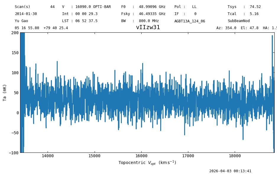
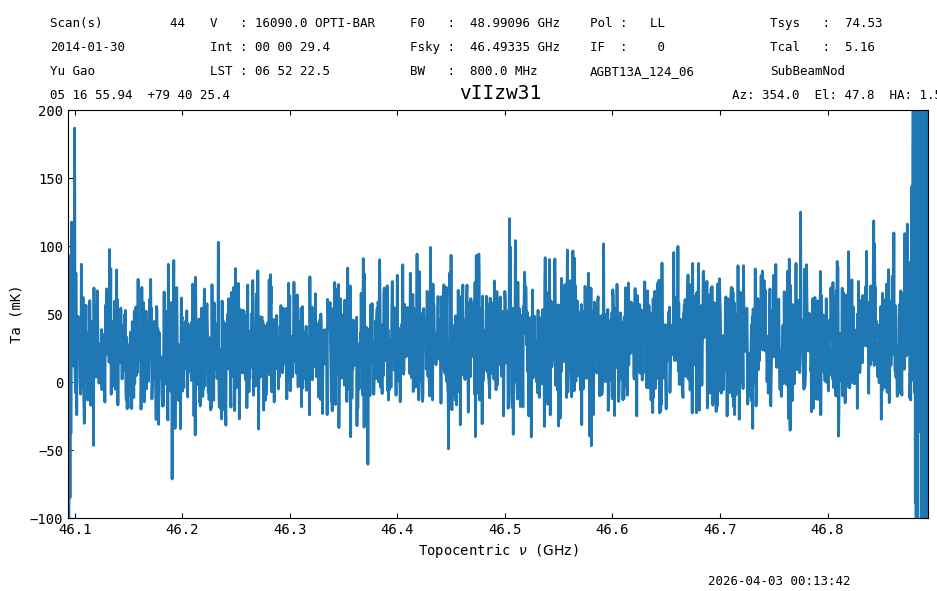
Plotting#
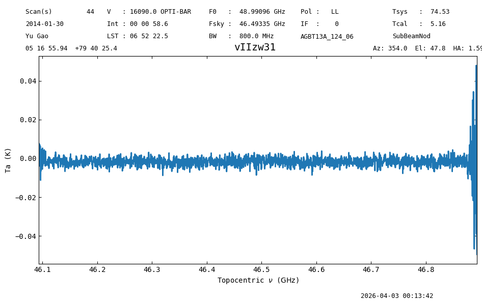
Plot the data and use different units for the spectral axis.
ta.plot(xaxis_unit="GHz");

ta.plot(xaxis_unit="km/s", yaxis_unit="mK", ymin=-100, ymax=200);
Calibration per Scan#
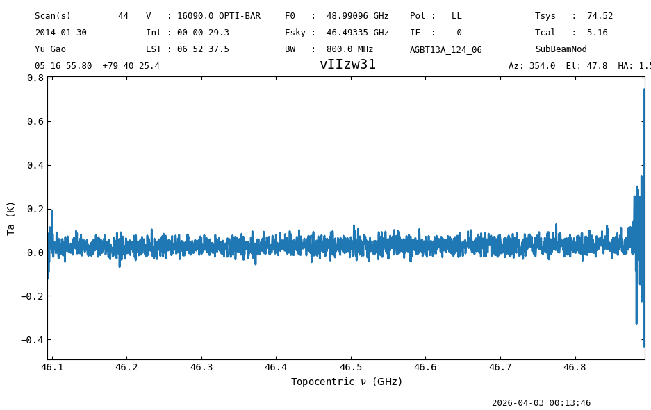
The second method (method="scan") of calibrating SubBeamNod scans reproduces the method of GBTIDL’s snodka.pro. This method treats the entire group of integrations as one cycle. It first time averages all of the integrations on source and off source, and then calibrates using the time averages.
sbn_scan_block2 = sdfits.subbeamnod(scan=44, fdnum=1, ifnum=0, plnum=0, method='scan')
ta2 = sbn_scan_block2.timeaverage()
ta2.plot(xaxis_unit="GHz", yaxis_unit="mK", ymin=-100, ymax=200);
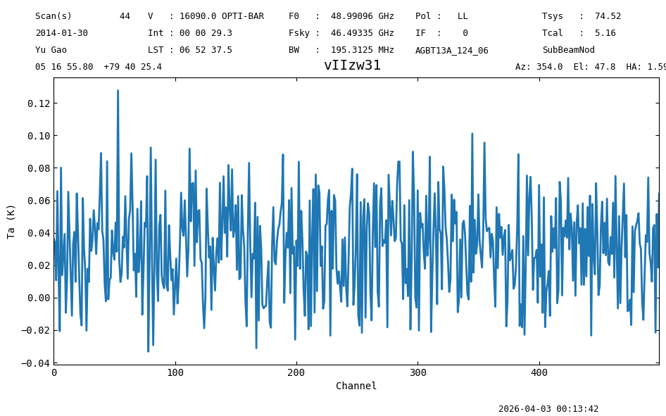
ta[250:750].plot(xaxis_unit="chan").spectrum.radiometer() # 1.2611058840974072
ta2[250:750].plot(xaxis_unit="chan").spectrum.radiometer() # 1.2630467493960695
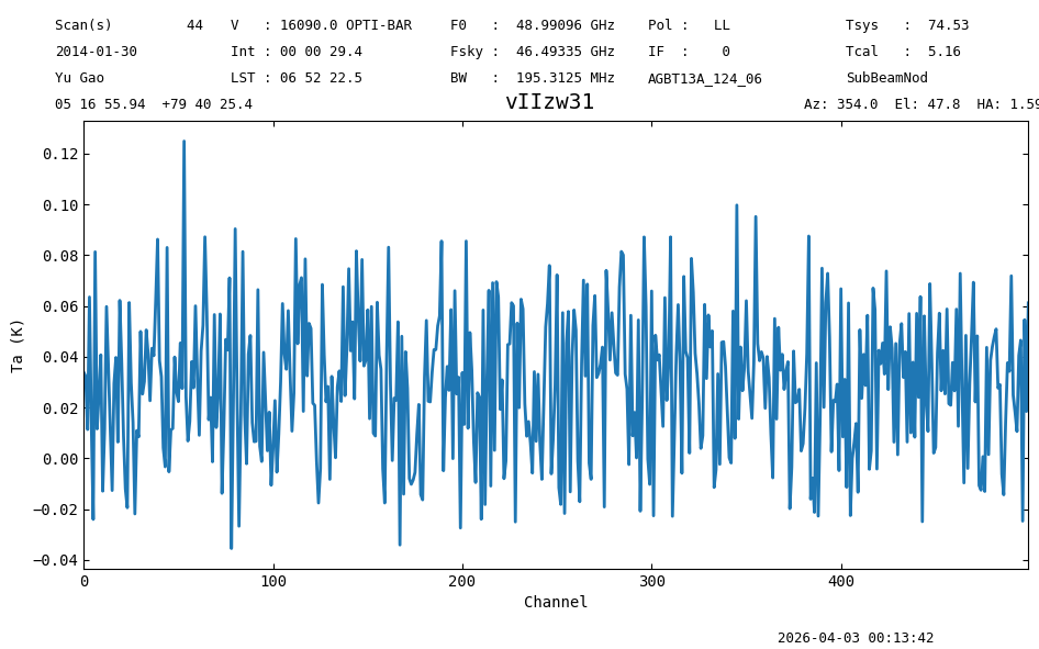
np.float64(1.263046749396072)
Compare the Two Methods#
(ta2 - ta).plot(xaxis_unit="GHz");
Using Selection#
We will repeat the calibration but using selection. First we pre-select the data to be calibrated using the sdfits.select() method.
sdfits.select(scan=44)
sdfits.selection.show()
 ID    TAG    SCAN # SELECTED
--- --------- ---- ----------
  0 9e6e10ff0   44       1600
After using selection, the calibration routines will only look for data matching the selection rules. It is also possible to add additional rules for a specific calibration, like the polarization number.
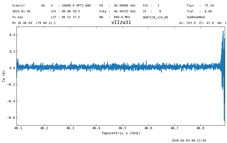
sbn_scan_block3 = sdfits.subbeamnod(plnum=0, fdnum=1, ifnum=0)
ta3 = sbn_scan_block3.timeaverage()
ta3.plot(xaxis_unit="GHz");
Polarization Average#
Now we will calibrate the other polarization and average the two polarizations together.
First we calibrate the second polarization, then time average it and finally we average them together.
sbn_scan_block4 = sdfits.subbeamnod(plnum=1, fdnum=0, ifnum=0)
ta4 = sbn_scan_block4.timeaverage()
pol_avg = ta3.average(ta4)
pol_avg.plot(xaxis_unit="GHz");
Final Stats#
Finally, at the end we compute some statistics over a spectrum, merely as a checksum if the notebook is reproducible.
pol_avg.check_stats(0.03836776)
00:13:50.083 I rms is OK (no unit was given, assumed K)
pol_avg[250:750].radiometer() # 1.2538633771107366
np.float64(1.2538633771107333)