SubBeamNod Data Reduction#
This notebook shows how to use dysh to calibrate an SubBeamNod observation via two different methods. It retrieves and calibrates SubBeamNod scans using GBTFITSLoad.subbeamnod() which returns a ScanBlock object.
from pathlib import Path
from dysh.util.download import from_url
from dysh.fits.gbtfitsload import GBTFITSLoad
Data Retrieval#
Download the example SDFITS data, if necessary.
url = "http://www.gb.nrao.edu/dysh/example_data/subbeamnod/data/AGBT13A_124_06/AGBT13A_124_06.raw.acs/AGBT13A_124_06.raw.acs.fits"
savepath = Path.cwd() / "data"
filename = from_url(url, savepath)
Data Loading#
Next, we use GBTFITSLoad to load the data, and then its summary method to inspect its contents.
sdfits = GBTFITSLoad(filename)
The returned sdfits can be probed for information.
You can also print a concise (or verbose if you choose verbose=True) summary of the data.
sdfits.summary()
| SCAN | OBJECT | VELOCITY | PROC | PROCSEQN | RESTFREQ | DOPFREQ | # IF | # POL | # INT | # FEED | AZIMUTH | ELEVATIO | |
|---|---|---|---|---|---|---|---|---|---|---|---|---|---|
| 0 | 44 | vIIzw31 | 16090.0 | SubBeamNod | 1 | 48.940955 | 48.990955 | 2 | 2 | 100 | 2 | 353.896698 | 47.758182 |
There is only one scan, using SubBeamNod. The scan is 44.
Data Reduction#
Single Scan#
To retrieve and calibrate a SubBeamNod scan we use sdfits.subbeamnod(). This method returns a ScanBlock, with one element per scan and per intermediate frequency.
Calibration per Cycle#
There are two different methods for calibrating a SubBeamNod scan. The first, with method="cycle" (the default) averages the data in each subreflector state for each cycle of integrations. That is, it separates the data into one signal/reference pair for each pair of subreflector states (on source and off source). Then calibrates each signal/reference pair independently and finally time averages the calibrated spectra.
sbn_scan_block = sdfits.subbeamnod(scan=44, fdnum=1, ifnum=0, plnum=0, method='cycle')
Time Averaging#
To time average the contents of a ScanBlock use its timeaverage method. Be aware that time averging will not check if the source is the same.
By default time averaging uses the following weights:
dysh these are set using weights='tsys' (the default).
ta = sbn_scan_block.timeaverage()
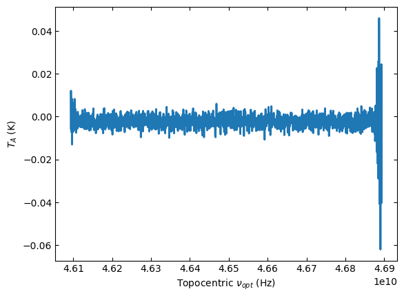
Plotting#
Plot the data and use different units for the spectral axis.
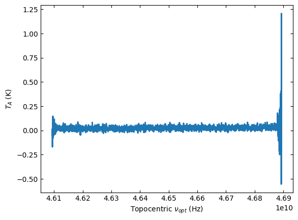
ta.plot()
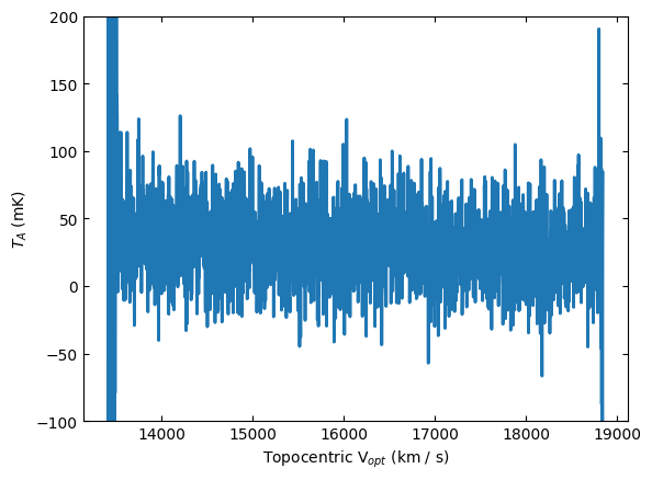
ta.plot(xaxis_unit="km/s", yaxis_unit="mK", ymin=-100, ymax=200)
Calibration per Scan#
The second method (method="scan") of calibrating SubBeamNod scans reproduces the method of GBTIDL’s snodka.pro. This method treats the entire group of integrations as one cycle. It first time averages all of the integrations on source and off source, and then calibrates using the time averages.
sbn_scan_block2 = sdfits.subbeamnod(scan=44, fdnum=1, ifnum=0, plnum=0, method='scan')
ta2 = sbn_scan_block2.timeaverage()
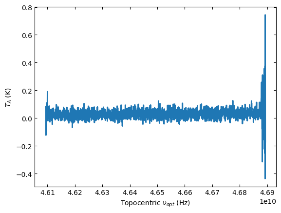
ta2.plot()
Compare the Two Methods#
(ta2 - ta).plot()
Using Selection#
We will repeat the calibration but using selection. First we pre-select the data to be calibrated using the sdfits.select() method.
sdfits.select(scan=44, fdnum=1, ifnum=0)
sdfits.selection.show()
 ID    TAG    SCAN IFNUM FDNUM # SELECTED
--- --------- ---- ----- ----- ----------
  0 fa62ac7cf   44     0     1        400
After using selection, the calibration routines will only look for data matching the selection rules. It is also possible to add additional rules for a specific calibration, like the polarization number.
sbn_scan_block3 = sdfits.subbeamnod(plnum=0)
ta3 = sbn_scan_block3.timeaverage()
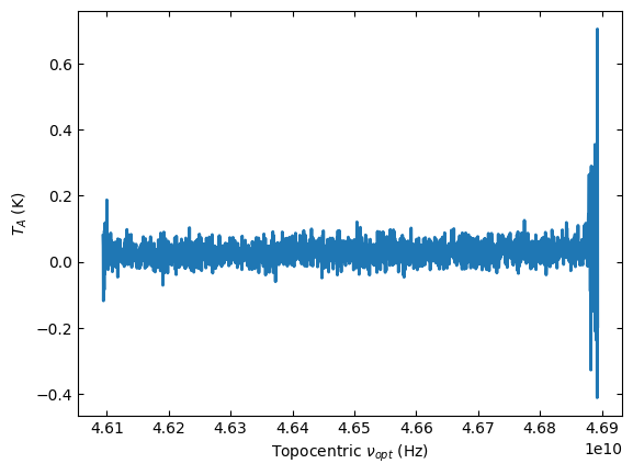
ta3.plot()
Polarization Average#
Now we will calibrate the other polarization and average the two polarizations together.
First we calibrate the second polarization, then time average it and finally we average them together.
sbn_scan_block4 = sdfits.subbeamnod(plnum=1)
ta4 = sbn_scan_block4.timeaverage()
pol_avg = 0.5*(ta3 + ta4)
pol_avg.plot()