Saving dysh data to external files#
This notebook gives examples of how to write out selected data from GBTFitsLoad and how to save
Spectrum,
Scan, and
ScanBlock to different formats.
from dysh.fits.gbtfitsload import GBTFITSLoad
from dysh.spectra.spectrum import Spectrum
from dysh.util.download import from_url
import matplotlib.pyplot as plt
import numpy as np
from pathlib import Path
Data Retrieval#
Download the example SDFITS data, if necessary.
url = "http://www.gb.nrao.edu/dysh/example_data/positionswitch/data/AGBT05B_047_01/AGBT05B_047_01.raw.acs/AGBT05B_047_01.raw.acs.fits"
savepath = Path.cwd() / "data"
filename = from_url(url, savepath)
Data Loading#
Next, we use GBTFITSLoad to load the data, and then its summary method to inspect its contents.
sdfits = GBTFITSLoad(filename)
sdfits.summary()
| SCAN | OBJECT | VELOCITY | PROC | PROCSEQN | RESTFREQ | DOPFREQ | # IF | # POL | # INT | # FEED | AZIMUTH | ELEVATIO | |
|---|---|---|---|---|---|---|---|---|---|---|---|---|---|
| 0 | 51 | NGC5291 | 4386.0 | OnOff | 1 | 1.420405 | 1.420405 | 1 | 2 | 11 | 1 | 198.343112 | 18.64274 |
| 1 | 52 | NGC5291 | 4386.0 | OnOff | 2 | 1.420405 | 1.420405 | 1 | 2 | 11 | 1 | 198.930571 | 18.787219 |
| 2 | 53 | NGC5291 | 4386.0 | OnOff | 1 | 1.420405 | 1.420405 | 1 | 2 | 11 | 1 | 199.330491 | 18.356075 |
| 3 | 54 | NGC5291 | 4386.0 | OnOff | 2 | 1.420405 | 1.420405 | 1 | 2 | 11 | 1 | 199.915725 | 18.492742 |
| 4 | 55 | NGC5291 | 4386.0 | OnOff | 1 | 1.420405 | 1.420405 | 1 | 2 | 11 | 1 | 200.304237 | 18.057533 |
| 5 | 56 | NGC5291 | 4386.0 | OnOff | 2 | 1.420405 | 1.420405 | 1 | 2 | 11 | 1 | 200.890603 | 18.186034 |
| 6 | 57 | NGC5291 | 4386.0 | OnOff | 1 | 1.420405 | 1.420405 | 1 | 2 | 11 | 1 | 202.327548 | 17.385267 |
| 7 | 58 | NGC5291 | 4386.0 | OnOff | 2 | 1.420405 | 1.420405 | 1 | 2 | 11 | 1 | 202.919161 | 17.494902 |
Calibrate a position switched scan.#
This returns a ScanBlock containing one PSScan with 11 integrations for the ON position and 11 integrations for the OFF position.
ps_scan_block = sdfits.getps(scan=51, ifnum=0, plnum=0)
print(f"Number of integrations = {ps_scan_block[0].nrows}")
Number of integrations = 22
Get the time average of the calibrated data#
This method returns a Spectrum.
ta = ps_scan_block.timeaverage()
ta.plot()
Reading and Writing Individual Spectra#
Inputs and Outputs#
dysh supports output to text files in a variety of formats familiar to users of astropy:
basic
commented_header
ECSV
fixed_width
IPAC
MRT
votable
fmt = [
    "basic",
    "commented_header",
    "ecsv",
    "fixed_width",
    "ipac",
    "mrt",
    "votable",
]
output_dir = Path.cwd() / "output"
for f in fmt:
    file = output_dir / f"testwrite.{f}"
    ta.write(file, format=f, overwrite=True)
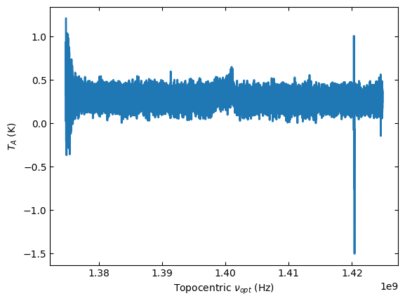
We can also write a spectrum to FITS format.
ta.write(output_dir / "testwrite.fits", format="fits", overwrite=True)
We can read spectra in FITS and a few formats. As noted in astropy, ECSV is the only ASCII format that can make a lossless output-input roundtrip and thus reproduce an original spectrum.
s1 = Spectrum.read(output_dir / "testwrite.fits", format="fits")
s1.plot()
s2 = Spectrum.read(output_dir / "testwrite.ecsv", format="ecsv")
s2.plot()
GBTIDL ASCII format#
dysh can read text files created by GBTIDL’s write_ascii function. However, those files do not provide sufficient metadata to fully recreate the spectrum. (For instance, they do not have complete sky coordinate information.)
url = "https://www.gb.nrao.edu/dysh/example_data/onoff-L/gbtidl-data/onoff-L_gettp_156_intnum_0_HEL.ascii"
filename_ascii = from_url(url, savepath)
s3 = Spectrum.read(filename_ascii, format='gbtidl')
print(s3, "\n", s3.meta)
Spectrum1D (length=32768)
Flux=[3608710. 3553598. 3604808. ... 3523171. 3545982. 3474847.] ct,  mean=493422767.43425 ct
Spectral Axis=[1.42009237 1.42009166 1.42009094 ... 1.39665654 1.39665582
               1.39665511] GHz,  mean=1.40837 GHz
 {'SCAN': 156, 'OBJECT': 'NGC2782', 'DATE-OBS': '2021-02-10 00:00:00.000', 'RA': 119.42083333333332, 'VELDEF': 'None-HEL', 'POL': 'YY'}
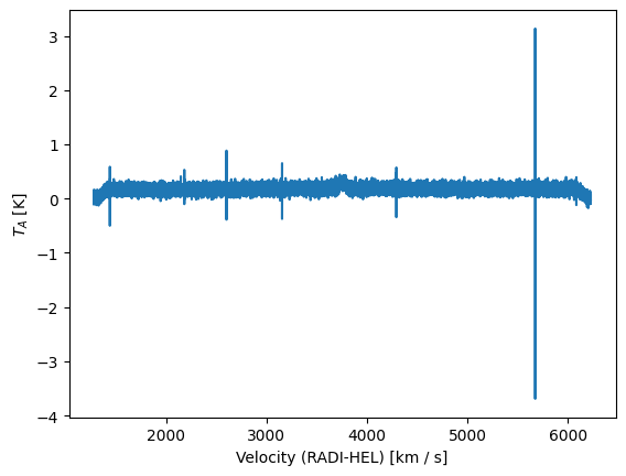
dysh can even read compressed ASCII files. Note these data have velocity on the spectral axis.
url = "https://www.gb.nrao.edu/dysh/example_data/onoff-L/gbtidl-data/onoff-L_getps_152_RADI-HEL.ascii.gz"
filename_ascii_gz = from_url(url, savepath)
s4 = Spectrum.read(filename_ascii_gz, format='gbtidl')
print(s4, "\n", s4.meta)
Spectrum1D (length=32768)
Flux=[-0.1042543   0.05250004  0.00432693 ... -0.05038555  0.03408394
       0.06139921] K,  mean=0.17345 K
Spectral Axis=[1281.15245599 1281.30342637 1281.45439674 ... 6227.69690405
               6227.84787443 6227.99884481] km / s,  mean=3754.57565 km / s
 {'SCAN': 152, 'OBJECT': 'NGC2415', 'DATE-OBS': '2021-02-10 00:00:00.000', 'RA': 114.65624999999999, 'VELDEF': 'RADI-HEL', 'POL': 'YY'}
Plot#
To plot the spectrum contained in the ascii files you have to use matplotlib.
plt.figure()
plt.xlabel(f"Velocity ({s4.meta['VELDEF']}) [{s4.spectral_axis.unit}]")
plt.ylabel(f"$T_A$ [{s4.flux.unit}]")
plt.plot(s4.spectral_axis, s4.flux)
[<matplotlib.lines.Line2D at 0x7fd36b93ba60>]
Writing Calibrated Data to SDFITS#
You can write the calibrated data from a ScanBlock in SDFITS format. If there are multiple Scans in the ScanBlock, they will all be written to the same binary table (useful for gbtgridder).
ps_scan_block.write(output_dir / "scanblock.fits", overwrite=True)
Writing out selected data from GBTFITSLoad#
The write() method of GBTFITSLoad supports down-selection of data. Data can be selected on any SDFITS column.
sdfits.write(output_dir / "mydata.fits", plnum=1, ifnum=[0,2],
             intnum=np.arange(100), overwrite=True, multifile=False)
 ID    TAG    IFNUM PLNUM               INTNUM              # SELECTED
--- --------- ----- ----- --------------------------------- ----------
  0 b3c22f4a6 [0,2]     1 [ 0  1  2  3  4...\n 96 97 98 99]        176
WARNING: AstropyDeprecationWarning: The update function is deprecated and may be removed in a future version.
        Use update_header instead. [dysh.fits.sdfitsload]
WARNING: AstropyDeprecationWarning: The update function is deprecated and may be removed in a future version.
        Use update_header instead. [dysh.fits.sdfitsload]
These data, can of course, be read back in.
sdfits2 = GBTFITSLoad(output_dir / "mydata.fits")
Writing SDFITS to multiple files#
If the data came from multiple files, for instance VEGAS banks, then by default they are written to multiple files, so
sdfits.write('mydata.fits')
would write to mydata0.fits, mydata1.fits, … mydataN.fits.
A future enhancement will preserve the A,B,C alphabetic extensions of the input data.