
Frequency-switched Data Reduction#
This notebook shows how to use dysh to calibrate a frequency switched observations. The idea is similar to an OnOff observation, except the telescope does not move to an Off in position on the sky, but moves its intermediate frequency in frequency space. Here we call the On and Off the Sig and Ref, but both will have the signal, just shifted in the band. Since the telescope is always tracking the target, combining the Sig and a shifted (folded) Ref, a \(\sqrt{2}\) improvement in signal-to-noise can be achieved.
The retrieval and calibration of frequency-switched observations uses GBTFITSLoad.getfs(), which returns a ScanBlock object.
from pathlib import Path
from dysh.util.download import from_url
from dysh.fits.gbtfitsload import GBTFITSLoad
Data Retrieval#
Download the example SDFITS data, if necessary.
url = "http://www.gb.nrao.edu/dysh/example_data/frequencyswitch/data/TREG_050627/TREG_050627.raw.acs/TREG_050627.raw.acs.fits"
savepath = Path.cwd() / "data"
filename = from_url(url, savepath)
Data Loading#
Next, we use GBTFITSLoad to load the data, and then its summary method to inspect its contents.
sdfits = GBTFITSLoad(filename)
sdfits.summary()
| SCAN | OBJECT | VELOCITY | PROC | PROCSEQN | RESTFREQ | DOPFREQ | # IF | # POL | # INT | # FEED | AZIMUTH | ELEVATIO | |
|---|---|---|---|---|---|---|---|---|---|---|---|---|---|
| 0 | 90 | W3OH | 0.0 | Track | 1 | 1.667359 | 1.667359 | 1 | 2 | 6 | 1 | 22.22828 | 18.114536 |
| 1 | 91 | W3OH | 0.0 | Track | 1 | 1.667359 | 1.667359 | 1 | 2 | 6 | 1 | 22.352097 | 18.20982 |
| 2 | 92 | W3OH | 0.0 | Track | 1 | 1.667359 | 1.667359 | 1 | 2 | 6 | 1 | 22.473876 | 18.304346 |
| 3 | 93 | W3OH | 0.0 | Track | 1 | 1.667359 | 1.667359 | 1 | 2 | 6 | 1 | 22.595308 | 18.399341 |
| 4 | 94 | W3OH | 0.0 | Track | 1 | 1.667359 | 1.667359 | 1 | 2 | 6 | 1 | 22.716326 | 18.494854 |
This data set contains 5 scans, 90 through 94. Each scan observed a single spectral window in two polarizations.
Data Reduction#
Single Scan#
The default is to fold the Sig and Ref to create the final spectrum. Use fold=False to not fold them and use_sig=False to reverse the role of Sig and Ref. We will start calibrating scan=90 (there are 5), ifnum=0 (there is 1) and plnum=1 (there are 2).
fs_scan_block = sdfits.getfs(scan=90, ifnum=0, plnum=1)
 ID    TAG    SCAN IFNUM PLNUM FDNUM # SELECTED
--- --------- ---- ----- ----- ----- ----------
  0 519c5298c   90     0     1   [0]         24
The return of sdfits.getfs is a ScanBlock which contains a single FSScan. The FSScan contains the calibrated data for all of the integrations. Now we will time average the integrations.
Time Averaging#
To time average the contents of a ScanBlock use its timeaverage method. Be aware that time averging will not check if the source is the same.
By default time averaging uses the following weights:
dysh these are set using weights='tsys' (the default).
ta = fs_scan_block.timeaverage(weights='tsys')
Plotting#
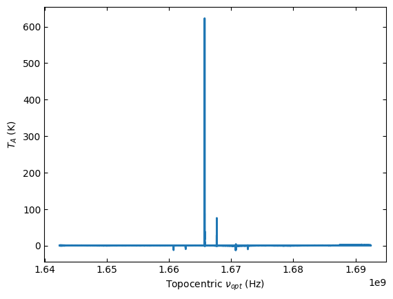
Plot the data and use different units for the spectral axis.
ta.plot()
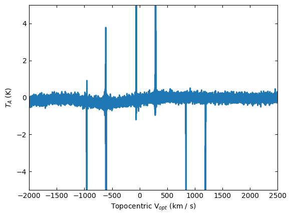
Now change the x-axis units to km s\(^{-1}\) and restrict the range being shown.
ta.plot(xaxis_unit="km/s", yaxis_unit="K", ymin=-5, ymax=5, xmin=-2000, xmax=2500)
Baseline Subtraction#
Next we remove a baseline from the data.
We zoom in into the baseline to determine which model the use.
ta.plot(xaxis_unit="chan", yaxis_unit="K", ymin=-2, ymax=2, title="before baseline subtraction")
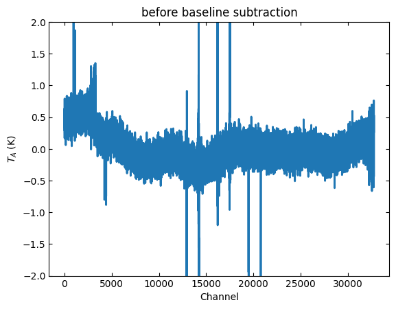
The baseline looks quasi-periodic, so a Chebyshev (model='chebyshev') polynomial model may be a good model to use. Other available alternatives are: hermite, legendre and classic polynomial
For baseline subtraction it is possible to specify the range of channels to be included in the fit (using the include argument) or excluded (using the exclude argument). Only one channel selection can be used at a time.
We will also look at the mean, rms, min and max of the data before and after baseline subtraction.
# Define a string.
fmt_str = "mean: {mean:.4f} median: {median:.4f} rms: {rms:.3f} min: {min:.2f} max: {max:.2f}"
# Print the statistics before baseline subtraction.
print(f"Before baseline subtraction -- {fmt_str}".format(**ta[4200:5300].stats()))

# Subtract the baseline.
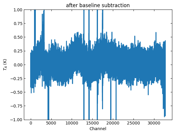
ta.baseline(model="chebyshev", degree=5, include=[(4200,10000),(22000,32000)], remove=True)

# Print the statistics after baseline subtraction.
print(f"After baseline subtraction -- {fmt_str}".format(**ta[4200:5300].stats()))

# Now plot the baseline subtracted spectrum.
ta.plot(xaxis_unit="chan", yaxis_unit="K", ymin=-1, ymax=1, title="after baseline subtraction")
Before baseline subtraction -- mean: 0.1734 K median: 0.1736 K rms: 0.140 K min: -0.88 K max: 0.60 K
After baseline subtraction -- mean: -0.0089 K median: -0.0085 K rms: 0.145 K min: -1.10 K max: 0.45 K
Now we will undo this baseline fit, and plot it again to see if we get the same spectrum back. Also adding the statistics on the first section of the baseline to confirm the statistics are all the same as before we started fitting.
ta.undo_baseline()
ta.plot(xaxis_unit="chan", yaxis_unit="K", ymin=-1, ymax=1, title='undo the baseline subtraction')
print(f"After undoing the baseline subtraction -- {fmt_str}".format(**ta[4200:5300].stats()))
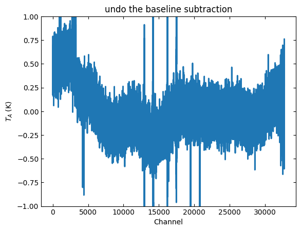
After undoing the baseline subtraction -- mean: 0.1734 K median: 0.1736 K rms: 0.140 K min: -0.88 K max: 0.60 K
output_dir = Path.cwd() / "output"
ta.savefig(output_dir / "baselined_removed.png")
Using Selection#
We will repeat the calibration of scan=90 and ifnum=0 using selection. To do this we pre-select the data using the sdfits.select() method.
sdfits.select(scan=90, ifnum=0)
fs_scan_block2 = sdfits.getfs(plnum=1)
ta2 = fs_scan_block2.timeaverage()
ta2.plot(title='Time averaged  plnum=1')
print(f"Using selection polarization 1 -- {fmt_str}".format(**ta2[4200:5300].stats()))
 ID    TAG    SCAN IFNUM PLNUM FDNUM # SELECTED
--- --------- ---- ----- ----- ----- ----------
  0 2d4fc8b75   90     0                     48
  1 5fe248907 [90]   [0]     1   [0]         24
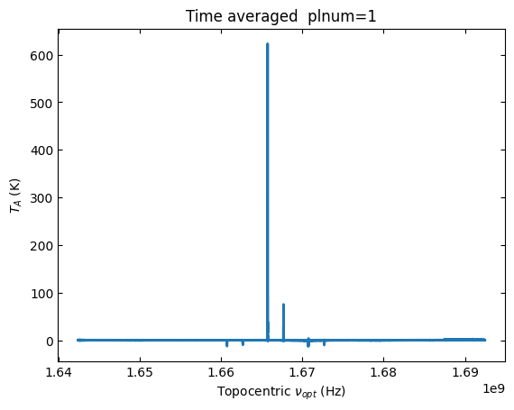
Using selection polarization 1 -- mean: 0.1734 K median: 0.1736 K rms: 0.140 K min: -0.88 K max: 0.60 K
Polarization Average#
Now we will calibrate the other polarization and average the two polarizations together.
First we calibrate the second polarization, then time average it and inspect the time-averaged calibrated spectrum.
fs_scan_block3 = sdfits.getfs(plnum=0)
ta3 = fs_scan_block3.timeaverage()
ta3.plot(title='Time averaged plnum=0')
print(f"Using selection polarization 0 -- {fmt_str}".format(**ta3[4200:5300].stats()))
 ID    TAG    SCAN IFNUM PLNUM FDNUM # SELECTED
--- --------- ---- ----- ----- ----- ----------
  0 2d4fc8b75   90     0                     48
  1 b224e0ea6 [90]   [0]     0   [0]         24
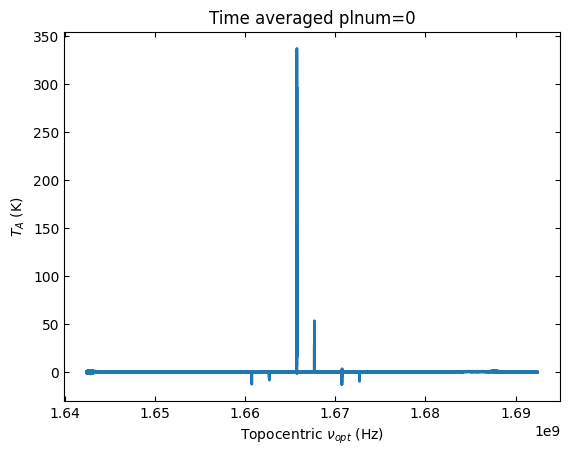
Using selection polarization 0 -- mean: 0.3231 K median: 0.3269 K rms: 0.135 K min: -0.42 K max: 0.81 K
Now we average the polarizations.
avg = 0.5*(ta2 + ta3)
avg.plot(ymin=-1,ymax=1, title='Averaged spectrum')
print(f"Polarization average -- {fmt_str}".format(**avg[4200:5300].stats()))
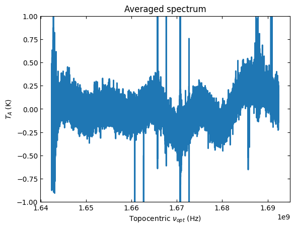
Polarization average -- mean: 0.2483 K median: 0.2515 K rms: 0.105 K min: -0.65 K max: 0.54 K
The noise is reduced by 1.34. Not exactly a factor of \(\sqrt{2}\), likely because of the baseline.