Spectral Axes, Velocity Frames and Conventions in dysh#
This notebook shows how to change spectral axes to represent different rest frames and Doppler conventions.
import astropy.units as u
from dysh.fits.gbtfitsload import GBTFITSLoad
from dysh.util.download import from_url
from pathlib import Path
Data Retrieval#
Download the example SDFITS data, if necessary.
url = "http://www.gb.nrao.edu/dysh/example_data/positionswitch/data/AGBT05B_047_01/AGBT05B_047_01.raw.acs/AGBT05B_047_01.raw.acs.fits"
savepath = Path.cwd() / "data"
filename = from_url(url, savepath)
Load the file#
sdfits = GBTFITSLoad(filename)
sdfits.summary()
/home/docs/checkouts/readthedocs.org/user_builds/dysh/envs/release-0.4.0/lib/python3.10/site-packages/astropy/time/formats.py:211: ResourceWarning: unclosed <socket.socket fd=52, family=AddressFamily.AF_INET, type=SocketKind.SOCK_STREAM, proto=6, laddr=('172.17.0.2', 36264), raddr=('192.33.116.7', 80)>
  self._select_subfmts(subfmt)
| SCAN | OBJECT | VELOCITY | PROC | PROCSEQN | RESTFREQ | DOPFREQ | # IF | # POL | # INT | # FEED | AZIMUTH | ELEVATIO | |
|---|---|---|---|---|---|---|---|---|---|---|---|---|---|
| 0 | 51 | NGC5291 | 4386.0 | OnOff | 1 | 1.420405 | 1.420405 | 1 | 2 | 11 | 1 | 198.343112 | 18.64274 |
| 1 | 52 | NGC5291 | 4386.0 | OnOff | 2 | 1.420405 | 1.420405 | 1 | 2 | 11 | 1 | 198.930571 | 18.787219 |
| 2 | 53 | NGC5291 | 4386.0 | OnOff | 1 | 1.420405 | 1.420405 | 1 | 2 | 11 | 1 | 199.330491 | 18.356075 |
| 3 | 54 | NGC5291 | 4386.0 | OnOff | 2 | 1.420405 | 1.420405 | 1 | 2 | 11 | 1 | 199.915725 | 18.492742 |
| 4 | 55 | NGC5291 | 4386.0 | OnOff | 1 | 1.420405 | 1.420405 | 1 | 2 | 11 | 1 | 200.304237 | 18.057533 |
| 5 | 56 | NGC5291 | 4386.0 | OnOff | 2 | 1.420405 | 1.420405 | 1 | 2 | 11 | 1 | 200.890603 | 18.186034 |
| 6 | 57 | NGC5291 | 4386.0 | OnOff | 1 | 1.420405 | 1.420405 | 1 | 2 | 11 | 1 | 202.327548 | 17.385267 |
| 7 | 58 | NGC5291 | 4386.0 | OnOff | 2 | 1.420405 | 1.420405 | 1 | 2 | 11 | 1 | 202.919161 | 17.494902 |
Data Reduction#
Next we fetch and calibrate the position switched data. We will use this data to show how to change rest frames and Doppler conventions.
psscan = sdfits.getps(scan=51, ifnum=0, plnum=0)
Create the time-averaged spectrum.
ta = psscan.timeaverage()
Example 1: Changing the x-axis of a spectrum plot#
Note this changes the axis of the plot but does not affect the underlying Spectrum object.
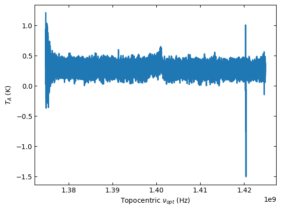
Default Rest Frame#
The default plot uses the frequency frame and Doppler convention found in the SDFITS file. In this case, that is topocentric frame and the optical convention.
ta.plot()
Change Rest Frame#
You can change the velocity frame by supplying one of the built-in astropy coordinate frames. These are specified by string name.
For example, to plot in the barycentric frame use "icrs". The change here is small, a shift of 22.8 kHz.
ta.plot(vel_frame='icrs')

In addition to the astropy frame names, we also allow 'topo' and 'topocentric'.
ta.plot(vel_frame='topo')
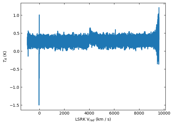
Doppler Convention#
One can also change the Doppler convention between radio, optical, and relativistic.
Here we also change the x-axis to velocity units and use LSRK frame.
ta.plot(vel_frame='lsrk', doppler_convention='radio', xaxis_unit='km/s')
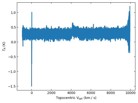
Finally, if you plot velocity units on the x-axis with no vel_frame given, it will default to the
frame decoded from the VELDEF keyword in the header if present.
ta.plot(xaxis_unit="km/s")
Example 2: Changing the spectral axis of the Spectrum.#
There are two ways to accomplish this. One returns a copy of the original Spectrum with the new spectral axis; the other changes the spectral axis in place.
A. Return a copy of the spectrum using Spectrum.with_frame()#
newspec = ta.with_frame('galactocentric')
newspec.plot()
print(f"The new spectral axis frame is {newspec.velocity_frame}")
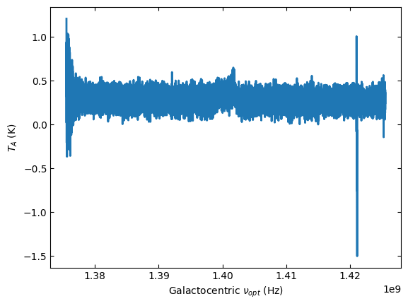
The new spectral axis frame is galactocentric
One can see that the spectral axis of the new spectrum is different.
ta.spectral_axis-newspec.spectral_axis
B. Change the spectral axis in place using Spectrum.set_frame()#
sa = ta.spectral_axis
ta.set_frame('gcrs')
print(f"Changed spectral axis frame to  {ta.velocity_frame}")
Changed spectral axis frame to gcrs
ta.plot()

Here the original the spectral axis has changed
ta.spectral_axis - sa
ta.target
<SkyCoord (FK5: equinox=J2000.000): (ra, dec, distance) in (deg, deg, kpc)
    (206.85210758, -30.40701531, 1000000.)
 (pm_ra_cosdec, pm_dec, radial_velocity) in (mas / yr, mas / yr, km / s)
    (4.68402043e-20, -4.68402043e-20, 4386.)>
ta.observer
<GCRS Coordinate (obstime=2005-06-27T02:05:58.000, obsgeoloc=(0., 0., 0.) m, obsgeovel=(0., 0., 0.) m / s): (x, y, z) in m
    (-3418483.37116048, -3651331.51587568, 3945691.32972075)
 (v_x, v_y, v_z) in km / s
    (-4.3110922e-08, 9.51169059e-08, 6.55464828e-08)>
Other useful functions#
Spectral Axis Conversion#
Convert the spectral axis to any units, frame, and convention with Spectrum.velocity_axis_to. dysh understands some common synonyms like ‘heliocentric’ for astropy’s ‘hcrs’.
ta.velocity_axis_to(unit="pc/Myr", toframe='heliocentric', doppler_convention='radio')
Spectral Shift#
Shift a spectrum in place to a given radial velocity or redshift with Spectrum.shift_spectrum_to
print(f"before shift {ta.spectral_axis}")
ta.shift_spectrum_to(radial_velocity=0*u.km/u.s)
print(f"after shift {ta.spectral_axis}")
before shift [1.42481735e+09 1.42481582e+09 1.42481430e+09 ... 1.37482191e+09
 1.37482038e+09 1.37481886e+09] Hz
after shift [1.44593293e+09 1.44593139e+09 1.44592984e+09 ... 1.39519657e+09
 1.39519502e+09 1.39519347e+09] Hz
Spectral Axis in Wavelengths#
The default is angstrom, use Quantity.to to convert to other units.
ta.wavelength.to('cm')
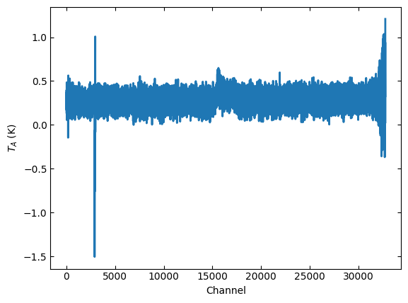
Plot in Channels#
Also, you can plot the x-axis in channel units
ta.plot(xaxis_unit='chan')