Working with GBT Position-Switched Data

Learning Goals

• Installing dysh using pip.

• Showing a summary of your data.

• Calibrating a position switched pais of scans using getps.

• Plotting the time averaged calibrated data.

Summary

In this tutorial you will learn how to use dysh to work with position switched data observed with the Green Bank Telescope (GBT).

The tutorial will walk you through how to install dysh, download a raw GBT SDFITS file using wget, and then use dysh to get a summary of the contents of an SDFITS file, calibrate the raw data and display it.

Tutorial

Installing dysh

You can install dysh using pip. From a terminal type

pip install dysh

After installing dysh you can start it by typing dysh in a shell. Alternatively, you can import it as any other Python module.

dysh

Downloading the raw data

In a Python instance, type

>>> import wget
>>> url = "http://www.gb.nrao.edu/dysh/example_data/onoff-L/data/TGBT21A_501_11.raw.vegas.fits"
>>> filename = wget.download(url)
>>> print(filename)
TGBT21A_501_11.raw.vegas.fits

Keep the Python instance open, we will start working with dysh now.

Note

The data used for this tutorial is ~800 MB. Make sure you have enough disk space and bandwidth to download it.

Inspecting the raw data

To import the relevant dysh functions type

>>> from dysh.fits.gbtfitsload import GBTFITSLoad

Now you will load the raw data and show a summary of its contents

>>> sdfits = GBTFITSLoad(filename)
>>> sdfits.summary(show_index=True)
    SCAN   OBJECT VELOCITY   PROC PROCSEQN  RESTFREQ   DOPFREQ # IF # POL # INT # FEED     AZIMUTH   ELEVATIO
0    152  NGC2415   3784.0  OnOff        1  1.617185  1.420406    5     2   151      1  286.218008   41.62843
1    153  NGC2415   3784.0  OnOff        2  1.617185  1.420406    5     2   151      1  286.886521  41.118134

Calibrating a position switched scan

The following lines will let you calibrate and time average the position switched pair of scans 152 and 153.

>>> psscan = sdfits.getps(scan=152, ifnum=0, plnum=0)
>>> ta = psscan.timeaverage(weights='tsys')

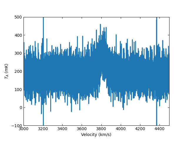
Plotting the calibrated data

>>> ta.plot(xaxis_unit="km/s", yaxis_unit="mK", ymin=-100, ymax=500, xmin=3000, xmax=4500)